Chapter overview
A large chip is built from blocks. Each block is closed on its own, then placed in the top level. Timing the top level with every block's full netlist is slow, and it needs a lot of memory.
Let us consider a chip with twenty blocks of two million cells each. That is forty million cells before the top-level logic is even counted. Yet the top-level paths only cross the block edges. The register-to-register paths deep inside each block were closed already by the block owners. Thus, most of the work in a flat run repeats checks that are already done.
A timing model is a smaller stand-in for a block. It keeps what the top level needs and drops the rest. This chapter covers the four model types in Tempus. They are the extracted timing model, the boundary model, the PTM and the interface logic model. They differ in what they keep, how accurate they are, and where you may use them.
The chapter matters for one more reason. A model is a summary, and a summary can be wrong. A wrong model hides real violations at the top level. Thus, we spend as much effort on checking models as on building them.
Learning objectives
- Explain why hierarchical flows need timing models, and what a model must reproduce.
- Explain which paths an extracted timing model (ETM) keeps and which it drops.
- Extract an ETM with
do_extract_model, and set every extraction global for a given goal. - Validate an ETM against the netlist with
write_model_timingandcompare_model_timing, and read the result. - Merge mode-specific ETMs into one multi-mode model, and select a mode at the top.
- Build and read a boundary model, and handle its clock mapping.
- Describe a block by hand with the PTM commands.
- Write, read and validate an interface logic model (ILM or XILM), and state its limits.
- Choose the right model for a given job.
Chapter roadmap
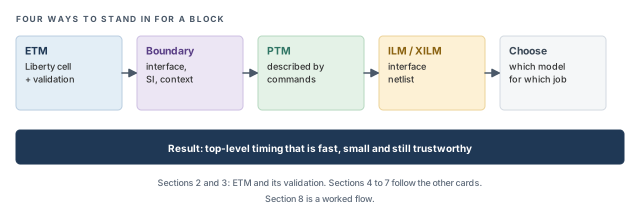
The chapter first explains why a block needs a model. It then covers one model type per section, and ends with how to choose. Figure 1 shows the order. Come back to it whenever you lose your place.
Key commands
Table 1 lists the commands covered in this chapter, grouped by section. Do not try to memorize them now. Each one is explained when it is first needed.
| Section | Command | What it does |
|---|---|---|
| 2 ETM | do_extract_model |
Extracts a Liberty timing model from the block |
| 2 ETM | merge_model_timing |
Merges mode-specific ETMs into one multi-mode model |
| 2 ETM | set_mode |
Selects one mode of a merged model at the top |
| 2 ETM | check_timing -check_only clock_gating_controlling_edge_unknown |
Finds MUX or XOR clock gating before extraction |
| 3 Validation | write_model_timing |
Writes slacks of the netlist or of the model |
| 3 Validation | compare_model_timing |
Compares the two slack reports with tolerances |
| 4 Boundary model | create_boundary_model, read_boundary_model |
Builds the model in the block run; loads it at the top |
| 4 Boundary model | create_glitch_boundary_model |
Builds a boundary model for glitch analysis |
| 5 PTM | create_ptm_model and the create_ptm_*, set_ptm_* family |
Describes a block's ports, arcs and rules by command |
| 5 PTM | report_ptm_model, save_ptm_model |
Reports and saves the described model |
| 6 ILM | write_ilm, specify_ilm, read_ilm |
Writes an ILM; names it and loads it at the top |
| 6 ILM | set_ilm_mode, unspecify_ilm, import_ilm_data |
Tunes, removes, or imports ILM data |
1 Why a block needs a timing model
1.1 The concept
A hierarchical flow times each block on its own first. The block owner closes setup, hold and design rules inside the block. The top level then uses each block as a single object. That object must still behave like the block at its pins. The data that describes this behavior is the timing model.
Think of a block as a sealed box with pins on the outside. The top-level engineer does not care what is inside the box. They care about three questions. When must a signal arrive at an input pin? When does an output pin change after the clock? How long does a signal take to pass straight through?
For example, a block input might feed a flop through 0.40 ns of logic. The flop needs 0.05 ns of setup. The top level does not need the gates on that path. It only needs one number. The input must arrive 0.40 + 0.05 = 0.45 ns before the clock edge at the flop.
1.2 Why it matters
A model makes the top-level run faster and smaller. On a large chip, this can decide whether a full signoff run finishes overnight or not at all.
However, a model is only as good as what it keeps. If it drops a path that matters at the top, a real violation can hide. If it keeps a pessimistic summary, the top level sees false violations and wastes ECO effort. Thus, every model must be checked, and used only where it is allowed.
1.3 The four model types
Table 2 compares the four types at a glance. The rest of the chapter explains each one.
| Model | What it keeps | Form | Typical use |
|---|---|---|---|
| ETM (extracted timing model) | Input-to-register, register-to-output and input-to-output timing as arcs | One Liberty cell | Fast top-level timing; block reuse |
| Boundary model (BM) | Interface logic, extended fanin, SI attackers, side loads and block context | A model directory | Top-level runs that need SI and PBA through the interface |
| PTM (prototype model) | Only what you describe by command | Commands, then a Liberty file | A block with no netlist yet |
| ILM / XILM (interface logic model) | Interface logic and the clock tree; XILM adds SI attackers | A model directory | Exploration; not for signoff in Tempus |
The "Form" column shows the main trade-off. An ETM and a PTM end as Liberty tables. A boundary model and an ILM keep real netlist. Tables are small and fast. Netlist is larger, but it lets the parent run detailed analysis such as crosstalk and path-based timing.
2 Extracted timing models (ETM)
2.1 The concept
An ETM turns a block into one Liberty cell. The cell has the same pins as the block. Inside, it has timing arcs instead of gates. Let us consider the block in Figure 2. It has four kinds of paths:
- in2reg – from an input port to a flop. It becomes a setup and hold check arc on the input pin, relative to the clock pin.
- reg2out – from a flop to an output port. It becomes a sequential clock-to-out arc.
- in2out – from an input straight to an output, with no flop in between. It becomes a combinational arc.
- reg2reg – from one internal flop to another. It is dropped.
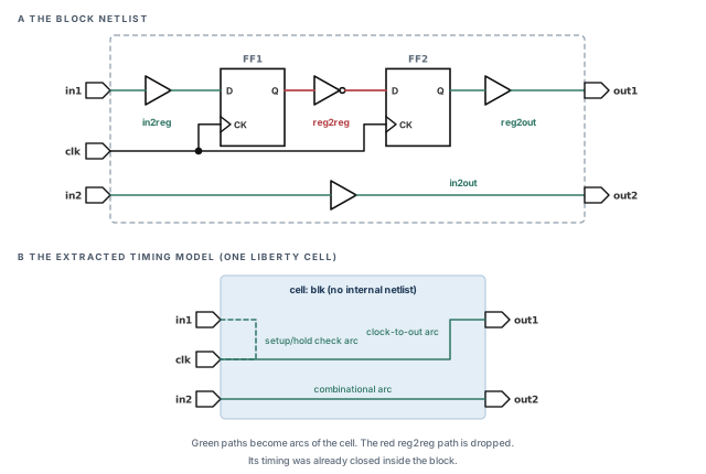
The reg2reg path is dropped because it never crosses the block boundary. Both its launch and capture flops are inside the block. The block run already closed it, and nothing at the top level can change it.
In other words, an ETM is the block as seen from the outside. Every arc in the cell answers one of the three questions from Section 1.
2.2 Context independence
The context of a block is everything the top level puts around it. It includes the slew arriving at each input, the load on each output, and the input and output delays in the constraints.
An ETM is meant to work in any top-level context. Its delay arcs are tables indexed by input slew and output load. Its check arcs are indexed by the data and clock slews. Figure 3 shows one such table. The top level supplies the slew and the load, and the table supplies the delay.
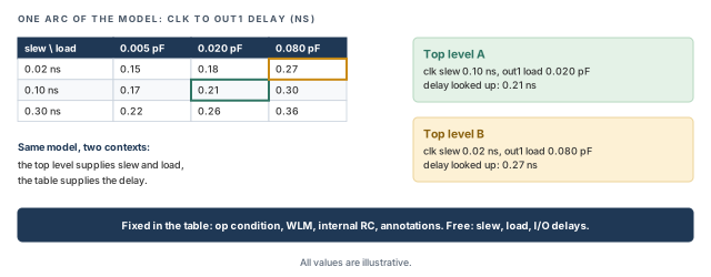
Thus, the model does not depend on the input slews, output loads or I/O delays used during extraction. That is what context-independent means here.
However, the model does depend on what was baked into the tables:
- the operating condition used during extraction,
- the wire-load model, if any,
- any annotations in the block run,
- the block's internal RC parasitics.
In other words, an ETM extracted at the slow corner describes the slow corner only. If the block's internal routing changes, the model must be extracted again.
A Liberty cell for an inverter is a good mental picture of an ETM. However, the picture fails in three places:
- An inverter cell is characterized once for a library. An ETM is extracted per block, per corner, and must be redone after any block change.
- An inverter has a handful of arcs. An ETM can have one arc per port pair, plus clock checks, which makes it large.
- An inverter's stage count is one. An ETM hides many stages inside one arc, which matters for AOCV later in this section.
2.3 Extracting the model
In an MMMC session, exactly one view must be active, as both the setup and the hold view. The reason is simple. One Liberty file describes one corner and one mode. If two views were active, the tool would not know which one to write.
tempus> set_analysis_view -setup {func_ss} -hold {func_ss}   ;# one view, both roles
tempus> do_extract_model test.lib \
          -verilog_shell_file test.v -verilog_shell_module test \
          -assertions test.asrt                              ;# model, shell, assertions
The options in this example do the following:
test.lib– the name of the Liberty model file to write.-verilog_shell_file test.v– also writes a Verilog shell, so a top-level netlist can instantiate the model.-verilog_shell_module test– names the module inside that shell.-assertions test.asrt– names the assertion files written next to the model.
Figure 4 shows what the extraction writes.
test.lib– the Liberty timing model.test.v– a Verilog shell: the module with its ports and no contents.test.asrt– assertions (constraints) for validating the model.test.asrt.latchInferredMCP– multicycle paths the tool inferred for latches.top_model.asrt– assertions for stitching the model into the top. Audit it; it is indicative only.
Without -assertions, the tool writes the default model.asrt and its .latchInferredMCP companion instead.
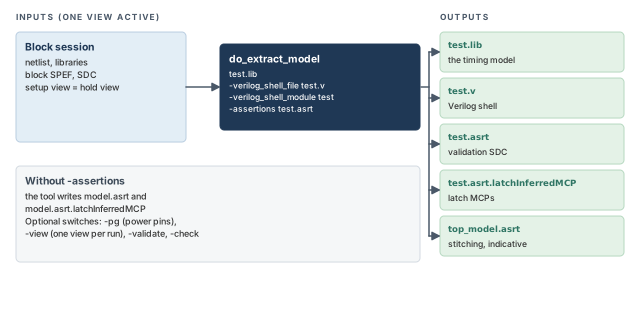
top_model.asrt is for stitching at the top and is only indicative – audit it before use.A beginner sources top_model.asrt into the top-level constraints without reading it. Its content is indicative only. It may duplicate or conflict with the top-level SDC. Always review it line by line before using any of it.
2.4 Extraction globals
Most extraction choices are made with globals, set before do_extract_model. A global set after extraction has no effect on the model already written. The globals fall into four groups.
Slews and clock checks
timing_extract_model_slew_propagation_mode–worst_slew(default) or a path-based mode. As the name suggests, withworst_slewthe tool carries the worst slew forward at each pin while building arcs. This is safe but can be pessimistic. The path-based mode follows each path's own slew, which is more accurate but has a limit described later in this section.timing_extract_model_write_clock_checks_as_arc true– recommended. It writes minimum pulse width and minimum period checks as slew-dependent arcs. The check then changes with the clock slew at the top, which is more realistic.- The companion global ending in
_as_scalar_tables– set totrueto write those clock checks as scalar tables instead. A scalar table typically holds one value, so it does not follow the clock slew at the top.
Constants, gating and DRV
timing_extract_model_case_analysis_in_library true– writes case-analysis constants as pin functions in the library. Whenfalse, the constants go in the assertion file instead. Choose one place and keep the top-level flow consistent with it.timing_extract_model_gating_as_nochange_arc false– writes clock-gating checks as setup and hold arcs, instead of no-change arcs. Use this when the top-level flow expects ordinary setup and hold checks on gating pins.timing_extract_model_consider_design_level_drv true– takes design-level DRV limits (such as max transition) into account in the model. Without it, a limit set on the design might not reach the model's pins.
Generated clocks, cycles and latency
timing_library_genclk_use_group_name true– names generated clocks in the library by their group name.timing_prefix_module_name_with_library_genclk– defaulttrue. It prefixes generated clock names with the instance name, as inINST/genclk1. The instance prefix typically keeps names unique when two instances of the model sit in one top level.timing_extract_model_disable_cycle_adjustment true– turns off cycle adjustment in the arcs. You must then apply the matching multicycle paths at the top. Otherwise the top-level check uses the wrong cycle.timing_extract_model_include_latency_and_uncertainty true– folds clock latency and uncertainty into the arcs.timing_extract_model_ideal_clock_latency_arc true– writes an arc for ideal clock latency.
Variation
timing_extract_model_aocv_mode–graph_based,path_basedornone(default). It decides whether and how AOCV derates are applied during extraction.timing_extract_model_write_lvf true– writes SOCV mean and sigma as LVF tables, so the top level can do its own statistical analysis. Withfalse, the tool folds sigma multiplier times sigma into the delay. The model then carries one fixed, already-derated number.
Let us consider the last global with numbers. Assume an arc with a mean of 0.20 ns, a sigma of 0.01 ns and a sigma multiplier of 3. With false, the model stores 0.20 + 3 × 0.01 = 0.23 ns. With true, it stores 0.20 and 0.01 separately. Thus, the true form keeps the statistics alive for the top level.
- For the exact name of the path-based slew mode value, use
help timing_extract_model_slew_propagation_modein your installation. - For the full name of the scalar-table global, use
helpon the clock-check globals.
2.5 Boundary nets and annotations
Two settings change what the model includes at its edges.
Boundary nets. A boundary net connects a block port to the first or last cell inside. With set_delay_cal_mode -ignoreNetLoad true, the model leaves out the load of these nets. You must then supply a boundary SPEF at the top. Otherwise those nets carry no load, and the delays at the block pins come out too small. Too-small delays can hide real setup violations. Figure 5 compares the two cases on one input net.
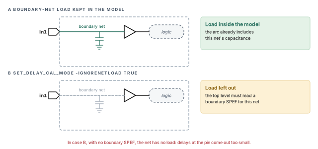
-ignoreNetLoad true, the load of the boundary net is not in the model, so the top level must supply it.What to notice: In case B the capacitor is grey: nothing in the model carries it any more.SDF annotation. Avoid it for extraction. SDF delays come from one context – one set of slews and loads. Baking them into the model defeats the purpose of a context-independent model. Annotated slews are ignored during extraction anyway.
2.6 Clocks inside the model
Clocks need extra care, because the model hides the clock tree. The top level sees only clock pins and arcs.
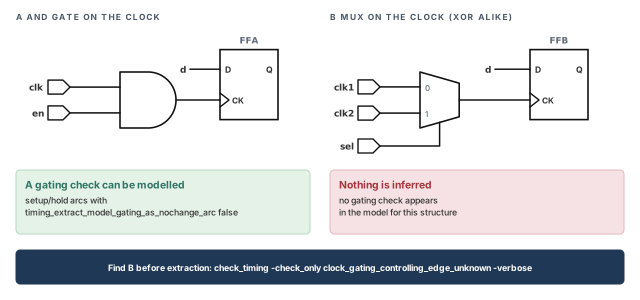
- Clock gating with a MUX or XOR. For these structures the tool infers nothing – no gating check appears in the model. Find them before extraction with
check_timing -check_only clock_gating_controlling_edge_unknown -verbose, then decide how each one must be checked. Figure 6 contrasts this with an AND gate on the clock. - Internal clock pins. A clock created on an internal pin appears in the library with
direction: internal. It is not one of the block's ports. - Several clocks on one master pin. Redefine the generated clock at the top with
-master_clock, so it uses the intended master. - Split clock pins. A clock can appear split into
<clk>_SEQ_pinand<clk>_COMB_pinnames. As the names suggest, these separate its sequential and combinational uses.
2.7 Table indices and output-to-output arcs
- Output-to-output arcs use 3-D tables, typically because their delay depends on more than one value. These arcs are off by default. They typically arise for ports joined by buffers. Confirm with
help do_extract_modelhow to turn them on if you need them. - By default, the table index points come from the first and last library cell used. The tool also prepends a 0 to each index, so the tables start at zero slew or load.
2.8 AOCV, power pins and SI
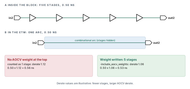
AOCV. Turn on AOCV with set_analysis_mode -aocv true. Then do_extract_model -include_aocv_weights writes the aocv_weight and clock_aocv_weight attributes. These weights typically tell the top level how many stages each arc stands for. A merged model keeps the minimum weight. Four cautions apply:
- Set the port stage weights in the block run, not at the top.
- One ETM may not fit several instances, because each instance sees a different context.
- Keep AOCV off while validating the model. Otherwise derates differ between the two sessions and hide real mismatches.
- If the top level uses design-level cell AOCV, give the ETM a cell table with derate 1.0. Otherwise the ETM's arcs can be derated a second time at the top.
Why do the weights matter? Figure 7 shows it with numbers. A five-stage path inside the block becomes one arc of 0.50 ns. Without a weight, the top can treat the arc as one stage and apply a large derate. With the weight, it can use the derate for five stages.
Power pins. do_extract_model -pg, with CPF or UPF loaded, writes voltage_map, pg_pin and the related_power_pin and related_ground_pin attributes. Use it when the top level runs multi-voltage analysis.
SI. Run SI analysis before extraction, so the arcs include crosstalk effects. An ETM cannot redo SI at the top, because its arcs are fixed tables.
2.9 Merging mode-specific models
A block often has a functional and a scan ETM. They have the same pins but different timing. Keeping two separate cells at the top is awkward. Figure 8 shows how they become one model.
merge_model_timing -library_file funct_etm.lib scan_etm.lib -modes funct scan \
  -mode_group funct_scan -outfile merged_funct_scan.lib   ;# one multi-mode model
Each option has one job:
-library_file– the ETMs to merge, in order.-modes– one mode name per input file, in the same order.-mode_group– the name of the mode group written into the library.-outfile– the merged Liberty file.
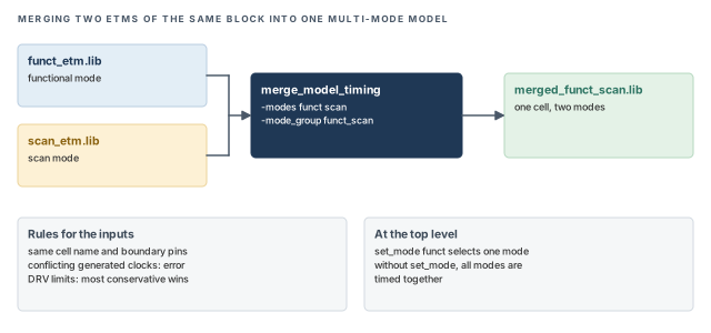
merge_model_timing combines models of the same cell into one library with named modes.What to notice: Without set_mode at the top, every mode is timed at once.At the top, select the mode with set_mode funct. Otherwise all modes are timed together, which mixes scan and functional arcs. The inputs must have the same cell name and boundary pins. Conflicting generated clocks cause an error. For DRV limits, the most conservative value is kept.
2.10 Limits of an ETM
- With path-based slew, the slews of side inputs are lost. Only the slew along the extracted path is kept.
- Only 2-D check arcs are supported.
- The stage count inside the block is hidden. Thus, AOCV at the top can pick the wrong derate, unless AOCV weights were written – see Figure 7.
A beginner extracts an ETM with SDF annotated and AOCV on, then validates it with AOCV still on. The model matches the block run but fails in a new context. Avoid SDF, and keep AOCV off during validation.
3 Validating an ETM
3.1 Why it matters
An ETM is a summary. A summary can be wrong – a global may be set badly, or a clock may be mapped wrongly. Before any top-level run trusts the model, its slacks must match the netlist's slacks on the same paths.
3.2 How it works
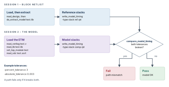
Validation uses two separate sessions, as Figure 9 shows.
- Session 1 loads the block netlist, extracts the model, and writes reference slacks from the netlist.
- Session 2 loads only the model, applies the validation assertions, and writes its own slacks.
compare_model_timinglines up the two reports path by path and flags mismatches.
Separate sessions matter. They prove the model works alone, with no hidden help from the netlist.
test.asrt, the validation assertions written during extraction.tempus> read_design blk_db test ;# load the block
tempus> do_extract_model test.lib -verilog_shell_file test.v \
-verilog_shell_module test -assertions test.asrt ;# extract
tempus> write_model_timing -type slack ref.rpt ;# reference slacks
tempus> exit ;# end session 1tempus> read_verilog test.v ;# the shell
tempus> read_lib test.lib ;# the model
tempus> set_top_module test ;# link
tempus> read_sdc test.asrt ;# validation assertions
tempus> write_model_timing -type slack comp.rpt ;# model slacks
tempus> compare_model_timing -ref ref.rpt -compare comp.rpt -outFile final.rpt \
-percent_tolerance 3 -absolute_tolerance 0.003 ;# compareThe read_design line uses illustrative names. Design Import covers its arguments.
The comparison options work as follows:
-ref– the reference report from the netlist.-compare– the report from the model.-outFile– the file that receives the comparison.-percent_tolerance– the allowed difference as a percentage, taken here relative to the reference slack.-absolute_tolerance– the allowed difference as an absolute time.
A path fails only if it breaks both tolerances. Let us consider a path with a reference slack of 0.200 ns and a model slack of 0.195 ns. The difference is 0.005 ns, or 0.005 / 0.200 = 2.5 percent. It breaks the 0.003 ns absolute tolerance. However, it stays inside the 3 percent tolerance. Thus, the path passes.
Now assume the model slack were 0.190 ns. The difference is 0.010 ns, or 5 percent. It breaks both tolerances, so the path fails.
While validating, set timing_prefix_module_name_with_library_genclk to false and timing_library_genclk_use_group_name to true. The generated clock names then match between the two sessions. Without this, every path on a generated clock can show up as a mismatch.
3.3 Validating several views
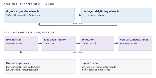
For MMMC, extract and write slacks once per view in session 1. Each view gets its own folder:
foreach v [list func_ss func_ff] {
  do_extract_model -view $v $v/test.lib -assertions $v/test.asrt   ;# per-view model
  write_model_timing -view $v -type slack -verbose               ;# per-view slacks
}
In session 2, repeat these steps for each view, as Figure 10 shows:
- Run
free_designto clear the previous view's model. - Load the shell and that view's model.
- Run
read_sdc $v/test.asrt.$vfor that view's assertions. - Run
compare_model_timingwith-ignore_view. As its name suggests, this stops differing view names in the two reports from counting as mismatches.
free_design clears the previous view first.What to notice: Session 2 reads $v/test.asrt.$v, the assertion file for that view.3.4 Built-in checks
do_extract_model -validate– validates as part of extraction. The validation directory is recreated each time. Thus, keep it apart from the ETM output, or the next run deletes your model.do_extract_model -check– runs Liberty sanity checks on the written model.
3.5 Exhaustive validation
The normal comparison checks the paths it reports. For extreme coverage, set timing_extract_model_exhaustive_validation_mode and timing_extract_model_exhaustive_validation_dir. Use the same settings at block and top. Results go to <outFile>_ev. This mode works with path-based slew only, and not together with -validate.
4 Boundary models
4.1 The concept
A boundary model keeps real netlist, not tables. It keeps everything that affects timing at the block's pins, as Figure 11 shows:
- the interface logic between the ports and the first or last flops,
- the extended fanin – logic that feeds the interface logic from inside the block,
- the SI attackers that couple onto the kept nets,
- the side loads hanging on interface nets,
- the block's context.
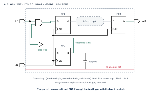
Why keep side loads and attackers that are not on the path? Because they change the path's delay. A side load adds capacitance to an interface net. An attacker adds crosstalk to it. Leaving them out would make the interface paths look faster than they are.
4.2 Why it matters
Because real netlist remains, the parent level can run SI and PBA through the block's interface. The parent computes crosstalk with real timing windows and re-times paths with real slews. An ETM cannot do this, because its arcs are fixed tables.
The cost is size. A boundary model is larger than an ETM and slower to load. However, it is usually much smaller than the full block.
4.3 Command breakdown
The block run creates the model. create_boundary_model runs update_timing itself, so it needs no separate timing command.
tempus> read_verilog block.v          ;# block netlist
tempus> read_libs slow.lib            ;# libraries
tempus> set_top_module block          ;# link
tempus> read_spef block.spef          ;# block parasitics
tempus> read_sdc block.sdc            ;# block constraints
tempus> create_boundary_model -dir bm ;# times the block, writes ./bm
At the top, the order matters. read_boundary_model must run before set_top_module, so the link step finds the model. Figure 12 lines up the two runs.
tempus> read_verilog top.v                ;# top netlist
tempus> read_lib slow.lib                 ;# libraries
tempus> read_netlist top.v -top top       ;# netlist with top named
tempus> read_boundary_model -dir bm       ;# before set_top_module
tempus> set_top_module top                ;# link
tempus> read_spef top.spef                ;# top parasitics, no block parasitics
tempus> read_sdc top.sdc                  ;# top constraints
tempus> update_timing ;# time the topThe block script uses read_libs and the top script uses read_lib. Confirm the exact command for your installation with help.
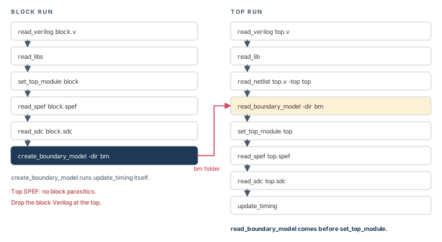
create_boundary_model writes the model; read_boundary_model reads it before set_top_module.What to notice: The red arrow is the only hand-over between the two runs: the bm folder.4.4 Common mistakes
- Block parasitics in the top SPEF. The top SPEF must not include the block's parasitics. The model already carries them, so they would be counted twice.
- Block Verilog still loaded. If both are present, the boundary model wins, but the run is costly. Drop the block Verilog from the top netlist list.
- SI settings. Use 2 SI iterations, and keep settings and CPF voltages consistent between block and top. Different settings make the model's context disagree with the parent's analysis.
4.5 Clock mapping
The top clocks must be mapped to the block clocks. The tool maps by waveform first, then by the same name. If neither works, you can give a mapping file with read_boundary_model -clock_mapping_file.
The tool writes two reports: <blk>_clock_map.txt and <blk>_unmapped_clocks.txt. Read both after every first run. An unmapped clock gives its nets unconstrained timing windows. Their handling then follows set_si_mode -unconstrained_net_use_inf_tw, covered in Signal Integrity Delay Analysis. Infinite windows can make crosstalk look worse than it is.
4.6 Glitch boundary models and MMMC
create_glitch_boundary_model -max_stagesbuilds a model for glitch analysis. The default is 2 stages. The output is<block>.db. More stages typically keep more logic for glitch propagation, at the cost of size.- For MMMC, run the block in CMMMC with the same views as the top, or a superset. A top view with no matching block view would typically have no model data.
set_top_module, and keep block parasitics out of the top SPEF.5 Prototype timing models (PTM)
5.1 The concept
Early in a project, a block may have no netlist yet. The top level still needs something to time against, so that top-level paths and budgets can be checked. A PTM is a model you describe by command: its ports, arcs and design rules. The tool then writes it out as a model the top level can read.
Let us consider a block dma. Its input data_in must be stable 0.3 ns before the clock edge and 0.1 ns after it. Its output data_out changes 0.05 ns after the edge. Figure 13 draws these three values.
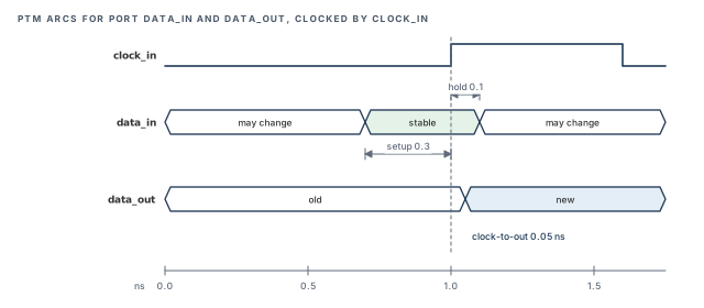
Assume a clock edge at 1.0 ns. Then data_in must be stable from 0.7 ns (1.0 − 0.3) to 1.1 ns (1.0 + 0.1). data_out changes at 1.0 + 0.05 = 1.05 ns. These numbers usually come from a budget, not from a measurement.
5.2 Command breakdown
The commands must start with create_ptm_model. The order below follows the example block.
tempus> create_ptm_model dma                                ;# first: start the model
tempus> set_ptm_global_parameter -param setup -value 1.5    ;# global setup value
tempus> create_ptm_drive_type -lib_cell INVX1 stdDrive      ;# drive type from a cell
tempus> create_ptm_load_type -lib_cell INVX4 stdLoad        ;# load type from a cell
tempus> create_ptm_port -type clock clock_in                ;# the clock port
tempus> create_ptm_port -type input data_in                 ;# an input port
tempus> create_ptm_port -type input bdis1                   ;# another input port
tempus> create_ptm_port -type output data_out               ;# an output port
tempus> set_ptm_port_drive -type stdDrive data_out          ;# output drive
tempus> set_ptm_port_load -value 4.0 bdis1                  ;# fixed load on a port
tempus> create_ptm_delay_arc -from clock_in -to data_out \
          -edge rise -value 0.05                            ;# clock-to-out
tempus> create_ptm_constraint_arc -setup -value 0.3 \
          -from clock_in -to data_in -edge rise             ;# setup
tempus> create_ptm_constraint_arc -hold -value 0.1 \
          -from clock_in -to data_in -edge rise             ;# hold
tempus> report_ptm_model                                    ;# review
tempus> save_ptm_model                                      ;# save
Figure 14 groups the whole family into nine steps. The list after it gives each command's job.
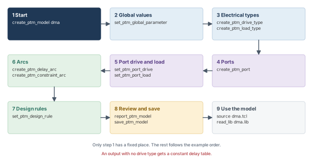
Each command in the family has one job:
create_ptm_model– starts the model and names it. It must come first, because every later command adds to it.set_ptm_global_parameter -param– sets a value for the whole model. It acceptssetup,holdandclk_to_output. The example also sets a 0.3 ns setup arc ondata_in. Confirm withhelphow a global value and an arc value combine.create_ptm_drive_type -lib_cell– defines a named drive strength, copied from a library cell. Output delays then change with load, as a real driver would.create_ptm_load_type -lib_cell– defines a named load, copied from a library cell's input. It also takes an optional-input_pin, for example-input_pin A.create_ptm_port -type– creates a port. It acceptsinput,output,inoutandclock. Typically, create every port before a later command names it. Buses are written like{data[31:0]}; the braces stop Tcl from treating[31:0]as a command.set_ptm_port_drive -type– attaches a drive type to an output port.set_ptm_port_load– sets the load of a port, either as a number with-valueor as a named type with-type stdLoad.create_ptm_delay_arc– a delay from one port to another, with-from,-to,-edgeand-value.create_ptm_constraint_arc– a check arc, here-setupor-hold, between a clock port and a data port.set_ptm_design_rule– sets-max_transition,-max_capacitanceor-max_fanouton ports given with-port, for example-port {bus[7:0]}.report_ptm_model– prints the model so you can review it before saving.save_ptm_model– writes the model out.
After saving, the example loads the model with source dma.tcl and read_lib dma.lib. Check the exact files written in your installation with help save_ptm_model.
An output with no drive type gets a constant delay table. Its delay then ignores the load, so a heavily loaded output looks as fast as a lightly loaded one. Give every output a drive type – and only one driver type per output.
Keep the PTM script under version control next to the block budget. When the budget changes, edit the script and regenerate the model. This keeps the numbers traceable.
6 Interface logic models (ILM and XILM)
6.1 The concept
An ILM keeps the block's I/O logic and its clock tree as real netlist. Everything else inside the block is removed. An XILM also keeps the SI attackers, with their timing windows stored in a .xtwf file. Figure 15 marks what each one keeps.
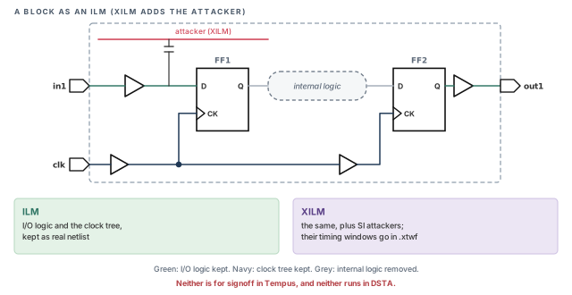
An ILM sits between an ETM and a boundary model. Like a boundary model, it keeps netlist, so path delays are computed at the top. Unlike a boundary model, it is not intended for signoff in Tempus.
ILMs are not for signoff in Tempus, and they are not supported in DSTA. Use them for exploration only – for example, quick top-level experiments before the final blocks arrive.
6.2 Command breakdown
The block run writes the model:
tempus> write_ilm -writeSDF -ignore_ports $ignorePorts \
-include_object $includeObjects -dir BlockB ;# ILM in ./BlockB-writeSDF– also writes delay data for the kept logic.-ignore_ports– ports whose logic need not be kept, such as static configuration inputs.-include_object– extra objects to keep even if they are not interface logic.-dir– the directory that receives the model.
The meanings of -writeSDF, -ignore_ports and -include_object above follow their names. Confirm them with help write_ilm.
At the top, the order matters, as Figure 16 shows.
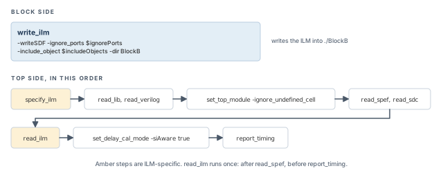
specify_ilm names the model before read_ilm, which runs once after read_spef.What to notice: The top netlist is linked with -ignore_undefined_cell, because the block module is empty there.tempus> specify_ilm -cell blockA -dir dir1 ;# before read_ilm
tempus> read_lib slow.lib ;# libraries
tempus> read_verilog top.v ;# top netlist
tempus> set_top_module TOP -ignore_undefined_cell ;# allow the empty block
tempus> read_spef top.spef ;# top parasitics
tempus> read_sdc top.sdc ;# top constraints
tempus> read_ilm ;# once, after read_spef
tempus> set_delay_cal_mode -siAware true ;# SI-aware delays
tempus> report_timing ;# after read_ilmThe order has a reason at each step:
specify_ilmtells the tool which cell is an ILM and where its data lives.- The libraries and the top netlist load next. The block module is empty, so linking uses
-ignore_undefined_cell. read_ilmruns once, afterread_spefand beforereport_timing. It replaces the empty block with the kept interface netlist.
6.3 Controls and rules
set_ilm_mode -keepHighFanoutPort falsegives better reduction, because high-fanout port logic is not kept.unspecify_ilmremoves a model named withspecify_ilm.- ILM settings are frozen after
read_ilm. Set them all before that command. - Message
ILM-334means the block module in the top Verilog is not empty. It must be empty, since the ILM provides its contents.
6.4 Importing ILM data without a database
When there is no saved block database, import the data in steps. The first step brings the netlist and setup; the next steps add parasitics and constraints:
tempus> import_ilm_data -si -dir d -cell c -mmmc -verilog x.v   ;# netlist and setup
tempus> import_ilm_data -incr -spef f -rcCorner rc              ;# add parasitics
tempus> import_ilm_data -incr -sdc f -viewName v                ;# add constraints
The -incr option adds data to what is already imported, instead of starting over. Confirm the details with help import_ilm_data.
6.5 MMMC and validation
- The MMMC names must match between top and block. A mismatched view name means no data for that view.
- Put the chip-level SDC in
-ilm_sdc_filesofcreate_constraint_modeorupdate_constraint_mode. timing_suppress_ilm_constraint_mismatches truehides constraint mismatches between top and block. It may also hide real errors, so use it only after reviewing the mismatches once.- To validate, run
write_ilm -dir ilm_dir -validation_dir vdir, thensource validation.src. The summary is invalidation.sum.
7 Choosing the right model
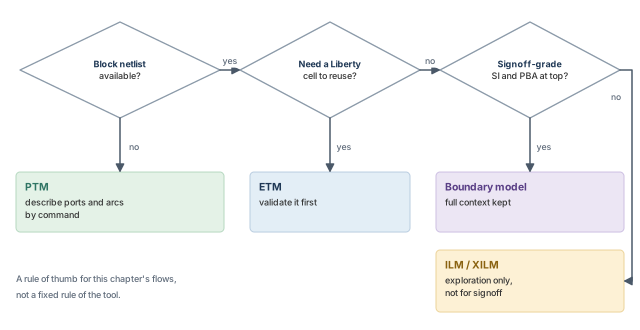
Each model answers a different need. Figure 17 gives a simple decision path.
- No netlist yet – PTM. It is fast to write, but only as good as its numbers. Replace it as soon as a netlist exists.
- A reusable Liberty cell – ETM. It is compact and fast. Validate it, and remember it is tied to one corner and one block version.
- SI and PBA through the interface at the parent – boundary model. It is larger, but it keeps the netlist the parent needs.
- Fast exploration – ILM or XILM. Useful for experiments, not for signoff in Tempus.
Let us consider a project timeline. In the first month, a new block exists only as a budget, so the top uses a PTM. Once the block netlist is stable, the owner ships an ETM with its validation report. Near tapeout, signoff runs need crosstalk across block edges, so the team switches to boundary models.
8 Worked example: an ETM for a block with two modes
The task. Block dma has a functional and a scan mode. The top team wants one Liberty model with both modes. We extract, validate and merge. The block is closed at the slow corner, and each mode has its own analysis view.
Step 1 – prepare the block run
Before extraction, we set the globals and look for clock gating the tool cannot infer.
# Assuming the dma block is loaded with its SPEF and SDC
tempus> set timing_extract_model_write_clock_checks_as_arc true   ;# recommended
tempus> set timing_prefix_module_name_with_library_genclk false   ;# for validation
tempus> set timing_library_genclk_use_group_name true             ;# for validation
tempus> check_timing -check_only clock_gating_controlling_edge_unknown \
          -verbose                                         ;# MUX/XOR gating
What to look for: the check_timing report should list no gating cells, or only ones you have reviewed. Any MUX or XOR gating left unexplained will have no check in the model.
Step 2 – extract one model per mode
Each mode is a separate view. One view is active at a time, as both setup and hold.
tempus> set_analysis_view -setup {func_ss} -hold {func_ss}   ;# functional view
tempus> do_extract_model funct_etm.lib -assertions funct.asrt ;# functional model
tempus> set_analysis_view -setup {scan_ss} -hold {scan_ss}   ;# scan view
tempus> do_extract_model scan_etm.lib -assertions scan.asrt   ;# scan model
What to look for: two Liberty files with the same cell name and the same pins. If the pins differ, the merge in Step 4 will fail.
Step 3 – validate each model
Run the two-session comparison from Section 3 for each model. Keep AOCV off while validating.
What to look for: final.rpt should show no failing paths. Assume one path shows a reference slack of 0.120 ns and a model slack of 0.090 ns. The difference is 0.030 ns, or 25 percent. It breaks both tolerances, so it fails. Trace that path's clock and gating before shipping the model.
Step 4 – merge
merge_model_timing -library_file funct_etm.lib scan_etm.lib -modes funct scan \
  -mode_group funct_scan -outfile merged_funct_scan.lib   ;# one model, two modes
At the top, the functional run uses set_mode funct. The scan run uses set_mode scan. Ship the merged model together with both validation reports.
- Step 1 uses
setfor the globals. Confirm the form your scripts use withhelpon each global. - The two generated-clock settings in Step 1 serve validation. If the top level holds several instances of the model, review whether the shipped model should keep the default instance prefix.
9 Common mistakes and how to catch them
Table 3 gathers the mistakes from this chapter. Each row gives the symptom you would see first.
| Symptom | Likely cause | Fix |
|---|---|---|
| ETM matches the block but fails at the top | SDF annotated during extraction | Extract without SDF |
| Validation fails on many paths | AOCV on during validation, or generated clock names differ | AOCV off; prefix false, group name true |
| Missing clock-gating checks in the model | MUX or XOR gating, nothing inferred | Find with check_timing -check_only clock_gating_controlling_edge_unknown |
| Boundary nets carry no load at the top | -ignoreNetLoad true and no boundary SPEF |
Supply the boundary SPEF |
| All modes timed together at the top | Merged model without set_mode |
Select the mode with set_mode |
| Merge fails | Conflicting generated clocks, or different pins | Use models of the same cell and boundary pins |
| ETM delays derated twice at the top | Design-level cell AOCV applied to the ETM | Give the ETM a cell table with derate 1.0 |
| Validation output deleted | -validate directory shared with the model |
Keep the validation directory apart |
| Boundary model run is slow | Block Verilog still loaded | Drop the block Verilog |
| Interface delays too large at the top | Block parasitics also in the top SPEF | Remove block parasitics from the top SPEF |
| Odd SI results with a boundary model | Unmapped clocks, infinite windows | Check <blk>_unmapped_clocks.txt; map the clocks |
ILM-334 at the top |
Block module in top Verilog is not empty | Empty the block module |
| PTM output delay ignores load | No drive type on the output | Set one drive type per output |
10 Interview preparation
It keeps in2reg, reg2out and in2out as arcs, and drops reg2reg.
- in2reg becomes a check arc, reg2out a sequential arc, in2out a combinational arc.
- reg2reg never crosses the boundary, and the block run already closed it.
Its arcs are tables indexed by slew and load, so they work under any top-level slews, loads and I/O delays.
- The top level supplies the lookup point; the table supplies the value.
- It still depends on operating condition, wire-load model, annotations and internal RC.
One, active as both the setup and the hold view.
- One Liberty file describes one corner and one mode.
- For several views, extract once per view with
-view.
compare_model_timing?Only when it breaks both the percent and the absolute tolerance.
- Take tolerances of 3 percent and 0.003 ns. A 0.005 ns gap on a 0.200 ns slack is 2.5 percent, so it passes.
- A 0.010 ns gap on the same slack is 5 percent and breaks both, so it fails.
SDF delays belong to one context, so the model loses its context independence.
- The model would carry delays for one set of slews and loads only.
- Annotated slews are ignored anyway.
The model hides the block's stage count, so the top cannot pick the right derate.
- Use
-include_aocv_weights, and set port stage weights in the block run. - Keep AOCV off during validation, and use a derate-1.0 cell table if design-level cell AOCV is used at the top.
set_mode?It times all modes together.
- Scan and functional arcs then mix, giving misleading results.
- Select one mode with
set_mode, for exampleset_mode funct.
Real interface netlist with extended fanin, side loads, SI attackers and context, so SI and PBA run at the parent.
- An ETM has fixed table arcs only, so it cannot redo crosstalk or path-based timing.
- The price is a larger model.
read_boundary_model go in the top script?Before set_top_module.
- The link step must find the model.
- Also keep block parasitics out of the top SPEF, and drop the block Verilog.
When the block has no netlist yet, so its ports and arcs are described by command.
- The values usually come from a timing budget.
- An output with no drive type gets a constant delay table.
No. ILMs are not for signoff in Tempus, and they are not supported in DSTA.
- XILM adds SI attackers but has the same limits.
- Use a boundary model when the parent needs signoff-grade SI and PBA.
Chapter recap
Key takeaways
- A timing model stands in for a block so the top level runs faster and smaller.
- An ETM keeps in2reg, reg2out and in2out as Liberty arcs and drops reg2reg. Extract with one active view.
- Set the extraction globals before
do_extract_model, and avoid SDF annotation. - Validate every ETM in two sessions. A path fails only if it breaks both tolerances.
- Merged ETMs need
set_modeat the top, or all modes are timed. - A boundary model keeps real interface netlist and context, so SI and PBA run at the parent.
- A PTM describes a block with no netlist; give every output one drive type.
- ILMs and XILMs are for exploration, not for signoff in Tempus.
Command recap
| Command | Purpose |
|---|---|
do_extract_model |
Extract an ETM (-assertions, -verilog_shell_file, -verilog_shell_module, -view, -pg, -include_aocv_weights, -validate, -check) |
write_model_timing, compare_model_timing |
Validate an ETM against its netlist |
merge_model_timing, set_mode |
Build and use a multi-mode ETM |
create_boundary_model, read_boundary_model |
Build and load a boundary model |
create_glitch_boundary_model |
Build a glitch boundary model |
create_ptm_model and family, report_ptm_model, save_ptm_model |
Describe, review and save a PTM |
write_ilm, specify_ilm, read_ilm |
Write and load an ILM |
set_ilm_mode, unspecify_ilm, import_ilm_data |
Tune, remove or import ILM data |
Compact glossary
| Term | Meaning |
|---|---|
| Timing model | A smaller stand-in that reproduces a block's timing at its pins |
| Hierarchical flow | Timing blocks first, then the top level with block models |
| ETM | Extracted timing model: one Liberty cell built from the block |
| in2reg, reg2out, in2out, reg2reg | Path types by where they start and end |
| Context | The slews, loads and I/O delays the top level puts around a block |
| Verilog shell | A module with ports and no contents |
| Boundary model | Interface netlist, extended fanin, attackers, side loads and context |
| Extended fanin | Logic inside the block that feeds the interface logic |
| Side load | A load hanging on an interface net |
| PTM | A model described by command, for a block with no netlist yet |
| ILM, XILM | Interface logic model; XILM adds SI attackers |
| Clock mapping | Matching top-level clocks to block clocks |
Practical perspective
On a real chip, the block owner usually delivers the model with the block. The top-level team trusts it only after seeing a clean validation report. Thus, a model without its validation is not a deliverable. It is better to ship the validation report next to the model, so anyone can check it.
It is also better to agree early on which model type each stage of the project uses. Switching model types late changes top-level results. That can trigger ECOs that were never needed, or hide ones that were.
What comes next
This chapter closes the series. We started at the prompt, with licenses and a scratch area. We then read a design, calculated delays and crosstalk, and modeled variation. We scaled to many views and many machines, fixed violations with signoff ECO, and finally shrank whole blocks into models. Each step answered one question: can this design be trusted to meet timing in silicon? Go back to any chapter whenever a run gives an answer you cannot explain.