Ch 4: Clock Tree Synthesis | PnR Flow

Part 1 — Orientation: what changes at CTS

The clock was a promise. Now you have to build it.

Every clock in your design has been a single line in a constraints file since the day you wrote the SDC. create_clock -period 0.625 [get_ports clk_core] tells the tool a clock exists, how fast it runs, and where it starts. It says nothing about how that clock physically reaches four thousand flip-flops scattered across a die. Until clock tree synthesis runs, the tool does not need to know. It assumes the clock arrives everywhere at once, with zero delay. That assumption is what this chapter takes away from you, on purpose.

Before CTS runs, the tool treats every clock as ideal: zero delay, zero skew, arriving at every register in the same instant. That is a useful fiction during placement and early optimization — it keeps the problem simple while cells are still moving. After CTS runs, the clock becomes propagated: a real physical net, buffered, routed, with a real insertion delay and a real difference in arrival time from one sink to the next. Everything you signed off against an ideal clock is now checked against a real one, and the numbers move.

New engineers hear "clock tree synthesis" and picture a separate, optional step. It is not optional and it is not separate from timing closure — it is the point where your timing closure stops being theoretical. Every setup and hold check you ran before CTS used a clock that does not exist yet. The moment clock_opt finishes, you find out whether the design you thought you closed is actually close to closed, or whether the ideal-clock fiction was hiding real problems. That is why CTS runs before routing, not after: you want to know the truth about your clocks while you still have room to react.

Where CTS sits in the flow

By the time you reach this chapter, placement is finished and legal — every cell sits on a real site, nothing overlaps, density is inside its target window. Routing has not started. CTS sits in that gap on purpose. The clock net is the one net in the whole design that cannot be allowed to take whatever routing resources signal nets leave behind, because every timing path in the design depends on it. So the clock gets built and routed first, on its own terms, with its own rules, before general routing ever begins.

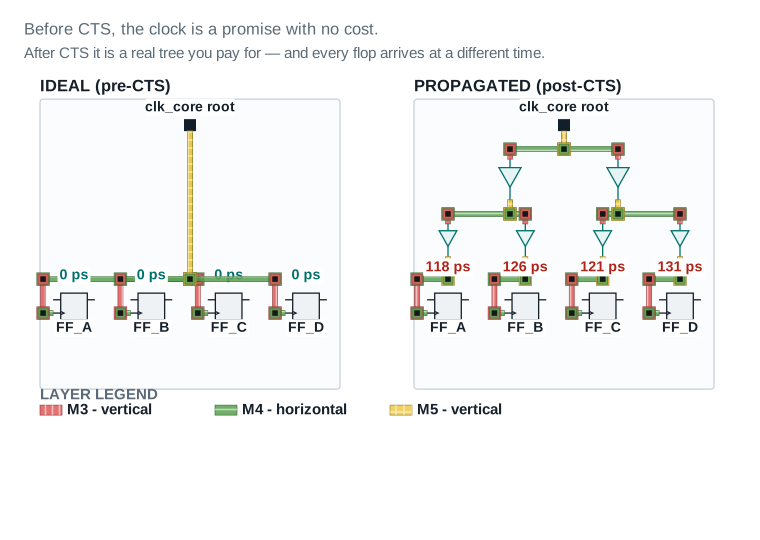
Two panels at identical coordinates. Left: clk_core reaching four flops as a single ideal net with zero delay. Right: the same four flops fed by a real buffer tree, with a different arrival time annotated at each flop. — Read it: Left panel, labelled IDEAL: `clk_core` reaches four real D flip-flop symbols — closed body, D and CLK pins on the left with the CLK edge-trigger triangle, Q on the right — as a single dashed net, every arrival time marked 0 ps and every instance name, FF_A through FF_D, printed directly beneath its own flop. Right panel, labelled PROPAGATED: the same four flops sit below a two-level buffer tree of real filled metal, and each flop's arrival time is different — 118, 126, 121 and 131 ps. Nothing about the logic changed between the two panels. Only the clock's physical reality did.

Cost ledger — ideal clock versus propagated clock
Insertion delay (ideal / real)	0 ps / 118-154 ps
Skew (ideal / real)	0 ps / 36 ps global
Buffer count (ideal / real)	0 / 38
Clock power (ideal / real)	0 mW / 2.1 mW (illustrative)

“Skew is the only thing that matters in CTS.” It is the number every beginner fixates on, because it is the one CTS-specific term they have heard before they ever open the tool. But a perfectly balanced tree with enormous latency is a bad tree. It burns more power, because every extra buffer level switches on every clock edge. It is more fragile to on-chip variation, because variation accumulates with every stage the clock passes through. And it makes hold fixing downstream harder, because a longer clock path gives the data path less room to be adjusted without breaking something else. Skew and insertion delay are a pair. Read both, every time.

The chapter's spine: three questions

Everything in this chapter answers one of three questions, and the chapter is organized around them in order:

What am I promising? Clock definitions, roots, endpoints, exceptions, design-rule constraints, and what the tool will and will not balance. Parts 2 through 4.
How do I build it? Synthesis, the clock_opt stages, the settings that actually matter, concurrent clock and data optimization, and multisource trees. Parts 5 through 8.
How do I prove it is real? Reading the reports, troubleshooting by symptom, a worked example end to end, and the handoff to routing. Parts 9 through 12.

Keep that shape in mind. Whenever a Part feels disconnected from the last one, it is answering a different one of the three questions, and that is deliberate.

The clock network typically touches every register in the block, and clock buffers alone can account for a meaningful share of total dynamic power on a high-frequency design — Nimbus‑8's own clock network runs close to a tenth of total dynamic power, a number this chapter's Dashboard 5 tracks explicitly. A clock tree you get wrong is not a local bug you fix with one ECO. It is a chip-wide cost that shows up in every power number and every timing report from here to tapeout.

Part 2 — Beginner foundations: the vocabulary, drawn

Every term, shown before it is named

This Part carries the most figures in the chapter, on purpose. A beginner is made or lost right here. Every term below gets drawn first and named second, because a definition you read before you have seen the thing is a definition you will misremember the first time it matters.

Skew: global and local

Skew is the difference in arrival time between two points on a clock network. That is the whole definition. The complexity is not in the definition — it is in which two points you mean.

Figure 2 — Skew, drawn: global versus local One root, one buffer level, four sinks with arrival times marked. Global skew dimensioned as the spread across all four sinks. Local skew dimensioned separately between two sinks that share a timing path.

Read it: Four real D flip-flop symbols, FF_A through FF_D named directly beneath each one, hang off one root through a single buffer level, arrival times 112, 148, 119 and 126 ps. Global skew is dimensioned across the full spread: 148 minus 112, 36 ps. A dashed teal line marks that FF_C and FF_D share a real timing path — a launch-capture pair — and local skew is dimensioned separately between just those two: 126 minus 119, 7 ps. The two numbers are not close, and that gap is the whole lesson.

Cost ledger — skew, drawn
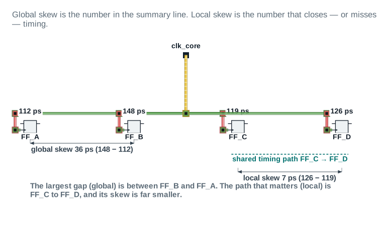
Global skew (max - min)	36 ps
Local skew, FF_C-FF_D shared path	7 ps
Sinks shown	4
Ratio local:global	~1:5 — global overstates the risk here

Global skew is the maximum minus the minimum arrival time across every sink in a clock or skew group. It is the number that shows up in a one-line QoR summary, and it is the number a review meeting asks about first, because it is easy to say out loud. Local skew is the arrival-time difference between two sinks that actually share a timing path — a launch flop and the capture flop it drives. Local skew is what determines whether that specific path meets setup or hold. Two sinks can have enormous global skew between them and never once appear together in a timing path, in which case that skew costs you nothing.

Insertion delay and latency

Insertion delay, sometimes called latency, is the time it takes the clock to travel from its root to a given sink. It is not free, and it does not trade cleanly against skew — you can always lower skew further by adding more buffer levels, but every level you add raises latency and adds more stages for on-chip variation to accumulate across.

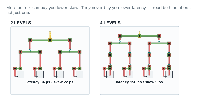
Left panel: a 2-level tree, latency 84ps, skew 22ps. Right panel: the same sinks with 4 levels, latency 156ps, skew 9ps. — Read it: Left, 2 levels: the root splits into 2 buffers, each fanning to 2 flip-flops -- latency 84 ps, skew 22 ps. Right, 4 levels: the same 4 branches continue through 2 more buffer stages each before reaching their flip-flops -- same 4 sinks, latency 156 ps, skew 9 ps. The extra depth buys 13 ps less skew for 72 ps more latency.

Cost ledger — insertion delay, and why it is not free
2 levels: skew / latency	22 ps / 84 ps
4 levels: skew / latency	9 ps / 156 ps
Buffer count, 2 vs 4 levels	6 vs 14 (illustrative)
OCV exposure	grows with every added level

“More buffer levels means a better balanced tree.” It usually does mean lower skew, right up until it does not — but it always means higher latency and more stages for variation to accumulate across. Every added level is a new place for on-chip variation to make one branch drift from another, which works against the very balancing you added the level to achieve. Add levels to fix a real skew problem you can point to. Do not add them by default because the tool has more knobs available.

Anatomy of a clock tree

One figure now carries every term this Part has introduced, plus the ones still to come, on a single picture you can point back to for the rest of the chapter.

Figure 4 — Anatomy of a clock tree Root, two levels of buffers, a clock-gating cell with its enable path marked, sink pins, one ignore pin drawn differently, and a leaf flop.

Read it: The clock root sits at the top. Three level-1 buffers fan out below it, teal triangles on real metal. Each drives two level-2 positions, six in total — five of the six are buffers; the sixth is an ICG, amber, its AND-gate body labelled CLK on the clock input and EN on its own dashed enable input, because that enable path carries its own timing check separate from the clock path. Below the level-2 row sit six real D flip-flop symbols, FF01 through FF06, each name printed directly beneath its own body so the six read unambiguously left to right: five are sink pins, FF06 is the ignore pin, reached through its own guide buffer and boxed in red dashed outline — the one your eye should land on last, because Figure 5 is about exactly that pin.

Cost ledger — anatomy of a clock tree
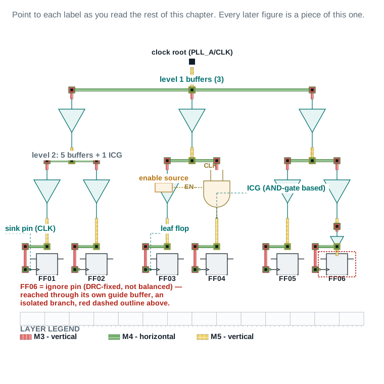
Levels shown	2
Buffers shown	8 (3 level-1 + 5 level-2)
Clock-gating cells	1 (ICG, own enable-path timing check)
Ignore pins shown	1 of 6 sinks

“A clock-gating cell is just another cell on the path.” It has its own enable input, and that enable input has its own timing check — the enable must be stable before the clock edge that would otherwise glitch through. Clock-gating cells are also where latency-driven splitting and collapsing decisions happen during optimization, because the tool can choose to merge or separate gated branches to improve balance. Treat every ICG in a tree as a decision point, not a pass-through buffer.

Sink pins versus ignore pins

Not every pin downstream of a clock root is treated the same way. A sink pin is a clock pin the tool actively balances against every other sink pin in its group. An ignore pin is one you have explicitly told the tool to exclude from balancing — usually because it sits behind a macro, in a different voltage domain, or on a path you are handling some other way.

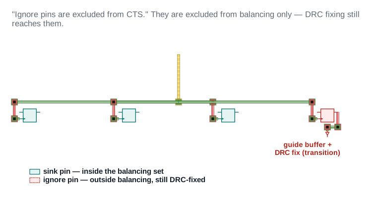
Same tree, two annotations. Three sink pins in teal, inside the balancing set. One ignore pin in red, outside the balancing set, with a guide buffer and a DRC fix drawn on the branch beyond it. — Read it: Four branches leave the root. Three end in teal boxes — sink pins, inside the balancing set. The fourth ends in a red dashed box — the ignore pin — and past it, a second red box marked "guide buffer + DRC fix (transition)" shows the branch continuing beyond the ignore point. That second box is the entire lesson of this figure: being ignored for balancing does not mean being ignored for design-rule fixing.

Cost ledger — sink pins versus ignore pins
Sinks balanced	3 of 4
Ignore pins (excluded from balancing)	1
DRC fixing on the ignore pin's branch	still applied (guide buffer)

“Ignore pins are excluded from CTS.” They are excluded from balancing, not from the tool's attention entirely. During clock tree synthesis the tool still adds a guide buffer at the ignore point and isolates the branch beyond it, and during subsequent optimization it still fixes any transition or capacitance violations on that isolated branch. What it will not do is spend effort trying to match that branch's arrival time against the rest of the tree. This distinction bites people who assume "ignored" means "untouched" — it does not.

Ignore pins exist because balancing is not always possible or desirable. A sink behind a hard macro, in a different voltage area, or feeding a scan-only path may simply be unreasonable to hold to the same skew target as everything else. Rather than let one awkward sink drag the whole balancing solution toward a worse compromise, you tell the tool to leave it alone for balancing purposes — and DRC fixing still keeps it electrically legal. That is a deliberate trade, not a gap in coverage.

Clock uncertainty, before and after

Before the clock tree exists, you have no real skew number to work with, so timing analysis uses clock uncertainty — a margin you set aside as a stand-in for skew you have not built yet. It is deliberately conservative, because guessing low would let real skew eat into your setup margin without warning.

A timing-window bar drawn to scale. Before CTS, an 80 picosecond uncertainty estimate occupies less than a third of the 260 picosecond period window. After CTS, the same 80 picoseconds splits into 28 picoseconds of measured skew and 52 picoseconds of margin returned, drawn at the same width as the original estimate. — Read it: Both rows are drawn on the same 260 ps period window (the light dashed outline), to the same scale. The top bar, BEFORE CTS, shows the 80 ps uncertainty estimate as the amber segment it actually is — under a third of the window, not the whole thing. The bottom bar, AFTER CTS, shows that same 80 ps once it is measured: 28 ps of it is real, remaining skew (red); the other 52 ps is margin handed back (teal, dashed) once the guess was replaced by a fact. The two rows' coloured segments are the same total width — nothing about the 80 ps changed except how much of it is still owed.

Cost ledger — clock uncertainty before and after CTS
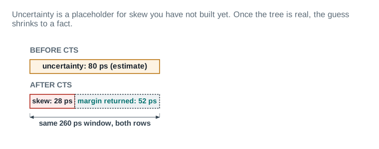
Uncertainty before CTS (estimate)	80 ps
Skew after CTS (measured)	28 ps
Margin returned to the data path	52 ps

Uncertainty before CTS is a tax every setup path pays, whether that path actually needs it or not. Once CTS gives you a real, measured skew number, you can replace the conservative estimate with the fact, and every path that was paying the estimated tax gets some of that margin back. This is exactly why timing so often looks like it "improves" right after CTS runs — not because anything got faster, but because a guess was replaced with a measurement, and the measurement was better than the guess.

Part 3 — Prerequisites and readiness

Four hard prerequisites, not four suggestions

The User Guide states this plainly on the page where Chapter 5 opens: before you run clock tree synthesis on a block, it should meet a short list of requirements. Every one of them is a hard prerequisite. None of them is a nice-to-have you can skip under schedule pressure and fix later — skipping any one of them costs you either runtime, quality of results, or both, and the cost shows up downstream where it is much more expensive to trace back.

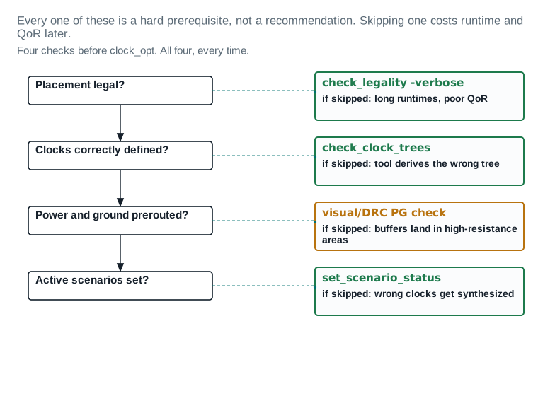
A vertical chain of four checks: placement legal, clocks defined, power and ground prerouted, active scenarios set, each with its check command and what happens if it is skipped. — Read it: Four boxes in a vertical chain, each with an arrow to the next. Placement legal, checked with `check_legality -verbose`, skip cost: long runtimes and reduced QoR. Clocks correctly defined, checked with `check_clock_trees`, skip cost: the tool derives the wrong tree. Power and ground prerouted, checked visually against DRC, skip cost: buffers land in high-resistance areas. Active scenarios set, checked with `set_scenario_status`, skip cost: the wrong clocks get synthesized. All four are hard prerequisites — there is no partial credit.

Cost ledger — prerequisites: what a clock tree needs first
Checks shown	4
Hard prerequisites (no partial credit)	4 of 4
Check commands named	4

Legal placement

Placement must be legal before CTS runs — every cell on a real site, nothing overlapping, nothing off-grid. Run check_legality -verbose and confirm zero violations. The User Guide is explicit that running clock tree synthesis on an illegally placed block can result in long runtimes and reduced quality of results. It also expects the estimated QoR for the block — congestion, timing, maximum capacitance, maximum transition — to already be acceptable before you start. If congestion issues are not resolved before CTS, the clock nets you are about to add will make congestion worse, not better.

“I can run clock_opt straight after placement.” You can type the command. Whether it does anything useful depends entirely on whether placement is legal and every clock is correctly defined first. Both are hard prerequisites, not soft recommendations, and the tool will not stop you from running clock_opt against an illegal or undefined design — it will just give you a bad tree, slowly, and you will spend more time debugging the result than you would have spent checking the prerequisite.

Power and ground prerouted

The power and ground network needs to be fully prerouted before CTS. Clock buffers, like every other cell, need a clean local supply, and buffer placement that ignores PG resistance can put buffers in locations with elevated voltage drop — a problem Part 6 revisits with the voltage-drop-aware clock_opt flow, but one that starts here, as a prerequisite that has to already be true.

Active scenarios and high-fanout nets

By default, the tool synthesizes and optimizes clocks in every active scenario enabled for setup or hold analysis. If the scenarios you actually care about — on Nimbus‑8, func_ss_0p72v_125c for setup and func_ff_0p88v_m40c for hold — are not the ones active, you build a tree optimized for the wrong conditions. High-fanout nets like scan enables should already be synthesized with buffers before CTS begins; CTS is not the place to first discover a thousand-fanout net with no buffering.

Every one of these four checks is cheap to run and expensive to skip. That asymmetry is the whole argument for treating them as gates, not suggestions. A check_legality -verbose run costs you seconds. A clock_opt run against illegal placement costs you an hour of runtime and a tree you have to throw away. Build the habit of running all four checks, every time, before you touch clock_opt — not because the manual says so, but because the cost of skipping one is never paid by you at the moment you skip it. It is paid later, by whoever debugs the result.

Confirm readiness, worked Verified

The four prerequisite checks, run against u_sens_tile before clock_opt touches clk_core.

1Confirm placement is legal:
```
icc2_shell> check_legality -verbose
```
2Confirm every clock is defined and derivable before you touch exceptions:
```
icc2_shell> check_clock_trees -clocks [get_clocks clk_core]
```

3Confirm the active scenarios match the signoff set:

icc2_shell> set_scenario_status func_ss_0p72v_125c -setup true -hold false
icc2_shell> set_scenario_status func_ff_0p88v_m40c -setup false -hold true

4Only after all three pass, proceed to Part 4's clock tree exceptions and Part 6's clock_opt.

check_clock_trees deserves its own close reading here, because it reappears constantly through this chapter and its job at this stage is specifically to catch problems before you have spent any effort defining exceptions or running synthesis. Called with no -clocks option it checks every clock in the current block; called with -clocks it scopes to the list you give it. It looks for clocks with no sinks, loops in the clock network, multiple clocks reaching the same register without multiple-clock propagation enabled, ignored exceptions, and several other structural problems — each with its own detailed man page explaining the fix. Run it here, before exceptions. Run it again in Part 4, after them.

Dashboard 1 — CTS readiness

clock_opt on an illegal placement or an undefined clock is not a fast failure. It is a slow one, days later, in a QoR review.

CTS readiness dashboard — is Nimbus‑8 ready for clock_opt? (part 1 of 2)
Item	Evidence	Source command / report	Threshold	Status	Required action
Placement legal and dense
1. Placement legal, whole block	0 illegal cells	`check_legality -verbose`	0 illegal cells	PASS	—
2. Density within target	81.9% utilization, within window	density report	78-84% target window	PASS	—
3. Congestion estimate acceptable	0 overflow gcells, worst-case pass	global route congestion estimate	0 overflow before CTS adds clock nets	PASS	—
Clocks defined and PG in place
4. All four clocks defined	clk_core, clk_dsp, clk_io, clk_pwr — 4 of 4	`report_clock -all`	4 of 4 clocks present	PASS	—
5. Clock sources identified	4 of 4 roots resolve to a real pin	`create_clock` / `create_generated_clock`	0 clocks with an unresolved source	PASS	—
6. Power and ground prerouted	100% of PG straps and rings routed	PG route report	100% prerouted before CTS	PASS	—
7. High-fanout nets already buffered	scan_enable, reset_n both pre-synthesized	netlist scan	0 unbuffered nets > 500 fanout	PASS	—

CTS readiness dashboard — is Nimbus‑8 ready for clock_opt? (continued — part 2 of 2)
Item	Evidence	Source command / report	Threshold	Status	Required action
Exceptions, cells and rules
8. Clock tree exceptions set and valid	6 exceptions defined, 0 flagged invalid	`check_clock_trees`	0 invalid exceptions	PASS	—
9. clk_pwr fanout into other domains	3 of 4 clock domains receive a clk_pwr-gated path	clock crossing report	flag for interclock balancing review	REVIEW	Confirm skew groups separate clk_pwr from the other three before build_clock; see Part 8.
10. Clock cell purposes set	CTS buffer/inverter set marked `-include cts`	`set_lib_cell_purpose`	Non-empty CTS cell list	PASS	—
11. Active scenarios set for setup and hold	func_ss_0p72v_125c (setup), func_ff_0p88v_m40c (hold)	`set_scenario_status`	Both signoff scenarios active	PASS	—
12. NDRs defined for clock nets	2x width rule defined on M3-M5	`set_clock_routing_rules`	Rule exists before route_clock	PASS	—

Readiness verdict: 11 PASS, 1 REVIEW, 0 BLOCKER → GO, with one item to close before build_clock.

Read it: Read gate 9 first — the only REVIEW. clk_pwr's fanout into the other three clock domains is exactly the interclock balancing problem Part 2 names, and it is worth watching before, not after, the tree is built.

Field values are this chapter's illustrative teaching data.

Part 4 — Defining the clock trees

What you are promising, made explicit

The tool derives a clock tree automatically from the clocks you defined in SDC — you do not have to hand-build a tree structure. What you do have to do is tell the tool about every exception to the default behaviour: pins that need special insertion delay, pins to exclude from balancing, and endpoints where balancing conflicts with something physical. This Part is where you make those promises explicit, one command at a time.

Deriving the clock trees

Before you touch a single exception command, analyze each clock tree in the block: what the root is, what the required sinks and exceptions are, whether the tree contains preexisting cells such as clock-gating cells, whether it converges with itself or with another clock tree, and whether it has timing relationships with other trees — interclock skew requirements, for instance. Nimbus‑8's clk_pwr, at 200 MHz, is exactly this last case: it crosses into all three of the other clock domains, which is why Dashboard 1 flagged it for review before the tree is ever built.

Clock tree exceptions: one command, three jobs

Every exception in this Part — insertion delay overrides, ignore pins, balancing conflicts — is set with the same command: set_clock_balance_points. It is worth being precise about this, because the wrong command name here is exactly the kind of mistake a beginner repeats for months once it is learned wrong.

“There must be a set_clock_tree_exceptions command for this.” There is not. It is a reasonable guess from the name of the topic — "Defining Clock Tree Exceptions" is literally the User Guide's section title — but no such command exists in the Tool Command Reference. Every exception in this section, insertion delay requirements and ignore pins alike, is set with set_clock_balance_points, and removed with remove_clock_balance_points. When the User Guide's section title and the actual command name disagree, the Tool Command Reference wins. Type the command that is actually in the TCR.

Defining insertion delay requirements

To override the default phase delay of zero for a sink pin, use the -delay option. The tool adds the value you specify, positive or negative, to the calculated insertion delay for path-delay calculations used to build the tree. By default it applies to both longest-path and shortest-path calculations, for both rising and falling edges; use -rise, -fall, -early and -late to scope it more precisely, and -corners to scope it to specific corners instead of all of them.

Insertion delay override, worked Verified

Specify a 2.0 ns insertion delay for rising-edge, earliest-path calculations at one sink pin, current corner only.

icc2_shell> set_clock_balance_points -clock [get_clocks clk_core] \
   -rise -early -delay 2.0 -balance_points [get_pins u_sens_tile/U2/CLK]

2Report what you just set:

icc2_shell> report_clock_balance_points -clock [get_clocks clk_core]

Defining ignore pins

To mark a pin as an ignore pin — excluded from balancing but still reached by the tree — use -consider_for_balancing false:

icc2_shell> set_clock_balance_points -clock [get_clocks clk_core] \
   -consider_for_balancing false -balance_points [get_pins u_sens_tile/U2/A]

During clock tree synthesis, the tool adds a guide buffer at that point and isolates everything beyond it from the rest of the balanced network — the mechanism Figure 5 drew in Part 2. During subsequent data-path optimization, the tool still fixes any DRC violations on the isolated branch. To remove an ignore-pin definition, use remove_clock_balance_points with the same -balance_points target.

Ensuring clock tree exceptions are valid

The tool identifies pins on the clock network using the is_clock_is_used_as_clock pin attribute during CTS. If you set an exception on a pin where that attribute is false — a pin the tool has already decided is part of the data network, not the clock network — the tool accepts the command without error, but silently ignores the exception during synthesis. This is a real trap, and it is specific: a command that appears to succeed and does nothing.

“The command ran with no error, so the exception took effect.” Not necessarily. set_clock_balance_points on a pin whose is_clock_is_used_as_clock attribute is already false is accepted syntactically and ignored functionally. If you want CTS to fix DRC violations further downstream than the default ignore point — say, all the way to a flop's data pin instead of just past a buffer — you have to explicitly name that further pin as the new ignore pin, and you have to verify with check_clock_trees afterward that the exception was not one of the ones silently ignored.

A placed region with a macro. Three sinks balance normally, one sits behind SRAM_MV1 in a separate voltage area and cannot be balanced against the other three. — Read it: Three sinks route cleanly to the left of the panel, each reachable in a direct path from the root — teal boxes, no conflict. A fourth branch runs along the top of the panel and terminates behind SRAM_MV1, drawn as a red dashed box, with a leader calling out "blocked by SRAM_MV1" and a note below explaining that it sits in a separate voltage area and cannot be balanced against the other three sinks. This is what a balancing conflict looks like as geometry, not as an abstract error message.

Cost ledger — clock tree exceptions on real geometry
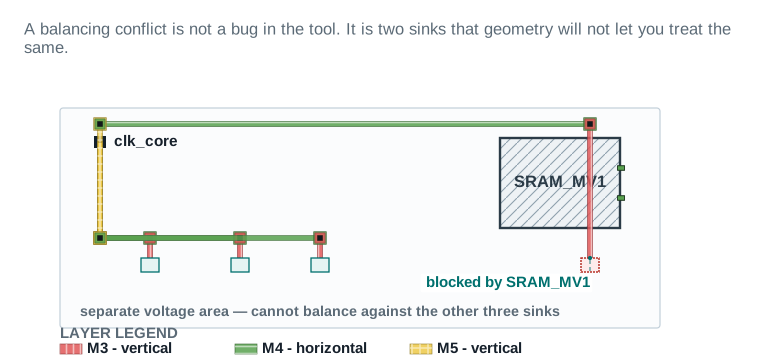
Sinks shown	4
Sinks in conflict (blocked by macro)	1
Cause	separate voltage area behind SRAM_MV1

Notice what the ignore-pin mechanism is actually doing: it is drawing an honest boundary around what the tool will promise to balance. A beginner's instinct is often to leave every sink in the balancing set and hope the tool figures out the hard cases on its own. It will not figure them out well — it will produce a worse compromise for every sink trying to accommodate the one it cannot reasonably match. Naming the hard case explicitly, as an ignore pin, gets you a better tree everywhere else, at the honest cost of one sink you handle separately.

Restricting optimization: don't-touch and size-only

Sometimes you want a cell in the clock network left alone entirely, or allowed to resize but never be replaced or removed. The don't-touch attribute and size-only restrictions give you that control on individual clock cells, and they matter most on preexisting structure — a clock-gating cell placed by RTL synthesis that you do not want CTS to rearrange, for instance.

Copying exceptions across modes

A multicorner-multimode design can have equivalent modes where the same exceptions should logically apply. Rather than re-entering every set_clock_balance_points call per mode, use set_clock_tree_options -copy_exceptions_across_modes -from_mode <mode> -to_mode <mode_list> to propagate them. This is the option most beginners never discover, and then wonder why their exceptions silently do not apply in a mode they forgot to set them in by hand.

Deriving exceptions from ideal latencies

If your design already carries ideal clock latencies — set with set_clock_latency on clock sink pins before CTS — you can convert those into equivalent set_clock_balance_points exceptions automatically, rather than re-deriving them by hand. This is common when a design inherits ideal-latency assumptions from an earlier, coarser stage of the flow and you want CTS to honor them as a starting point instead of discarding them.

Verifying with check_clock_trees

Run check_clock_trees a second time here, after every exception is set, not just once before you started. It checks for the same structural issues as before, plus — for multicorner-multimode designs — conflicting per-clock exception settings and conflicting balancing settings across active scenarios. Every message it produces has its own detailed man page explaining the fix; read it before guessing.

Re-verify after exceptions, worked Verified

icc2_shell> check_clock_trees -clocks [get_clocks clk_core] -include_ccd_checks

2Fix every reported issue manually before proceeding to Part 5 or Part 6.

Setting clock tree design rule constraints

Beyond balancing, the tree also has to respect electrical design rules — maximum transition and maximum capacitance on clock nets, typically tighter than the equivalent limits on data nets, because clock nets drive many loads and any edge degradation compounds across the whole tree. These are set with set_max_transition -clock_path and set_max_capacitance -clock_path, scoped to the clock objects rather than the whole design, and with set_clock_tree_options for skew and latency targets that Part 5 covers in depth.

Dashboard 2 — clock definition board

Every later figure and report in this chapter names one of these four clocks. This is the one table that defines them all in one place.

Clock definition board — the four clocks, side by side
Item	Evidence	Source command / report	Threshold	Status	Required action
The four clocks
1. clk_core — 1.60 GHz, u_sens_tile	root PLL_A/CLK, 4,210 sinks, 38 ignore pins	`report_clock_settings -clocks clk_core`	target skew 40 ps / target latency 160 ps	PASS	—
2. clk_dsp — 1.10 GHz, u_dsp_core	root PLL_B/CLK, 3,340 sinks, 21 ignore pins	`report_clock_settings -clocks clk_dsp`	target skew 55 ps / target latency 210 ps	PASS	—
3. clk_io — 800 MHz, u_io_ring	root PLL_C/CLK, 980 sinks, 6 ignore pins	`report_clock_settings -clocks clk_io`	target skew 70 ps / target latency 240 ps	PASS	—
4. clk_pwr — 200 MHz, u_pwr_ctrl	root PLL_D/CLK, 640 sinks, 14 ignore pins, fans into 3 other domains	`report_clock_settings -clocks clk_pwr`	target skew 90 ps / target latency 300 ps	REVIEW	Interclock conflict with clk_core/clk_dsp/clk_io at the gated boundary; see Dashboard 1 row 9.
Exceptions applied
5. clk_core exceptions	1 ignore-pin group (behind SRAM_MV1), 0 conflicts	`set_clock_balance_points`	0 unresolved conflicts	PASS	—
6. clk_dsp/clk_io/clk_pwr exceptions	5 ignore-pin groups total, 0 conflicts	`set_clock_balance_points`	0 unresolved conflicts	PASS	—

Definition verdict: 4 of 4 clocks fully defined, 1 conflict outstanding (clk_pwr) → proceed, with clk_pwr flagged.

Read it: Compare row 1 (clk_core) against row 4 (clk_pwr): clk_core has the tightest skew target and the most sinks, and it is the tree this chapter follows end to end in Figures 17A-17E.

Sink counts and targets are this chapter's illustrative teaching data.

Part 5 — Settings that actually matter

Ten settings out of thirty

The User Guide lists roughly thirty settings under clock tree synthesis options. This Part does not restate that list. A beginner who reads thirty options in a row remembers none of them. Instead, here are the eight or ten a beginner will actually set on a real project, why each one exists, and a pointer to the manual for the rest.

A chapter that lists thirty options and explains none of them in depth teaches nothing — it just relocates the manual's table of contents into a different document. A chapter that picks ten and explains why each exists, with a worked example, teaches something you can actually use on Monday morning. The other twenty settings are real and sometimes necessary, but you will look them up when you have a specific problem that needs them. You will not remember them from a first read, and pretending otherwise wastes your time and mine.

1. Which cells CTS may use

set_lib_cell_purpose -include cts <lib_cell_list> tells the tool which library cells are valid choices for clock tree synthesis. Without a deliberate purpose list, the tool may reach for cells that are technically legal but not meant for clock duty — low-drive cells that would need an unreasonable number of stages, or cells whose characterization was never validated for clock-tree use. Setting this once, early, at the library level is worth more than debugging a strange buffer choice three stages into a build.

2 and 3. Target skew and target latency

set_clock_tree_options -target_skew <value> sets the required maximum skew for a clock; the default is 0, which the tool interprets as "minimize skew," not literally zero. -target_latency <value> sets a minimum early insertion delay constraint — there is no default, and you only set it when you specifically need a floor on how fast the clock is allowed to arrive, which matters more often than beginners expect on designs with hold-sensitive I/O timing.

Target skew and latency, worked Verified

Set clk_core's skew target to 40 ps, the value Dashboard 2 records.

icc2_shell> set_clock_tree_options -clocks [get_clocks clk_core] \
   -target_skew 0.040

4. Optimizing for local skew, not just global

Because global skew and local skew are different numbers — Part 2's whole point — the tool needs to know which one you want it optimizing toward on a per-clock or per-group basis. Skew groups, discussed next, are the mechanism for this; the setting itself lives on the target-skew and target-latency options scoped to a skew group rather than a whole clock.

5. Primary corner

Multicorner-multimode designs synthesize and optimize across every active scenario by default, but one corner is treated as primary for certain decisions during tree construction. Confirm which corner is primary before a build, especially when your setup and hold signoff scenarios sit at very different voltage and temperature corners, as Nimbus‑8's func_ss_0p72v_125c and func_ff_0p88v_m40c do.

6. Clock cell spacing rules

Clock buffers are often given minimum spacing rules relative to one another and relative to other cells, to reduce coupling and keep clock cells from clustering in a way that creates local congestion or IR-drop hot spots. This is a placement-adjacent setting that pays off specifically on high buffer-count trees, which on Nimbus‑8 means clk_core more than the other three.

7. Skew groups

A skew group is a named subset of a clock's sinks that you want balanced against each other and reported on separately from the rest of the clock. Skew groups are how you tell the tool "these sinks matter to each other; that sink over there does not need to match them." set_clock_tree_options -skew_groups <name> -target_skew <value> and the matching -target_latency option are the two you will use most.

8. Name prefix for clock cells

Every buffer and inverter CTS inserts gets a name, and by default that name follows a tool-chosen prefix. Setting a project-specific prefix — something that reads clearly as "CTS put this here" in a later netlist diff or ECO review — is a small setting with an outsized payoff the first time someone has to distinguish a CTS-inserted buffer from a hand-placed one months later.

9. NDRs on clock nets

Non-default routing rules — wider metal, tighter spacing, or explicit shielding — are set on clock nets with set_clock_routing_rules, scoped by -clocks or -nets and by -net_type (root, internal, or sink). Figure 10, in Part 6, shows exactly what this buys you physically. Set it before route_clock runs; it has no effect applied afterward.

Skew groups are worth a second pass, because they are the setting beginners most often skip and most often need. A single clock with a hundred sinks does not need one skew group covering all hundred with an identical target — it usually needs a handful of groups, each covering the sinks that genuinely share timing paths with each other. Set target skew per group, not per clock, once your sinks are large enough in number that a single number stops making sense for all of them.

10. Power-reduction settings

clock_opt.flow.enable_clock_power_recovery, set to either power or area, controls whether the final_opto stage spends its recovery pass minimizing clock power or clock area. Part 6 covers the mechanics; the setting itself belongs on this list because it is the one power-related option a beginner should set deliberately rather than leave at whatever the tool defaults to.

These ten settings are the ones that show up in almost every real CTS runsheet, across almost every project. The other twenty exist for specific situations — a particular library quirk, a particular multivoltage structure, a particular power-recovery edge case — and you reach for them when that situation actually arises, with the manual open. Memorizing all thirty in advance is not a skill; knowing which ten to set by default and where to look for the rest is.

Part 6 — Building it: clock_opt and what happens inside

One command, three stages, each a checkable thing

Everything in Parts 2 through 5 was preparation. This is where the tree actually gets built. Two commands can do it: synthesize_clock_trees, which only synthesizes and optimizes the tree itself, and clock_opt, which synthesizes, routes, and further optimizes the whole design against the tree it just built. On a real project, you use clock_opt.

Standalone synthesis versus clock_opt

synthesize_clock_trees builds and optimizes clock trees from the clock definitions, skew-driven, and can optionally also optimize for slack. It takes a -clocks option to scope which clocks to compile, a -propagate_only option that just propagates already-built clocks without rebuilding them — useful when new scenarios are activated after CTS already ran — and postroute options for re-optimizing an already-routed tree. It is a building block. clock_opt is the command you actually run for a full CTS pass, because it also handles routing and the optimization that depends on real, routed parasitics.

The three stages

clock_opt runs three stages in sequence: build_clock, route_clock, and final_opto. You can limit execution to a contiguous range with -from and -to; if you omit -from it starts at build_clock, and if you omit -to it runs through final_opto.

build_clock synthesizes and optimizes the clock trees for every clock in every mode of every active scenario. After this stage, the synthesized clocks are set as propagated — the ideal-clock fiction from Part 1 is gone from this point forward.
route_clock detail-routes the synthesized clock nets. Before this stage, the tree exists only as a logical structure with estimated, unrouted timing.
final_opto performs further optimization, timing-driven placement, and legalization, then runs a full global route on the whole block and follows it with extensive global-route-based optimization — incremental legalization and route patching included.

Figure 9 — The clock_opt stages

Read it: Panel 1, build_clock: two buffers and three real D flip-flop symbols, named FF1, FF2 and FF3 directly beneath their own bodies, connected by dashed guide lines — the tree exists logically, nothing is routed. Status strip below reads built yes, routed no, legal no. Panel 2, route_clock: the same structure, now real filled metal on real layers. Status strip: built yes, routed yes, legal no. Panel 3, final_opto: identical geometry, now with a teal band across the bottom marked "legalized + global routed" and on-grid legalization ticks beneath each flop. Status strip: built yes, routed yes, legal yes. Each stage's output is a checkable fact, not a vague sense of progress.

Cost ledger — the clock_opt stages
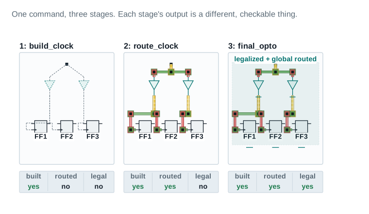
build_clock: built / routed / legal	yes / no / no
route_clock: built / routed / legal	yes / yes / no
final_opto: built / routed / legal	yes / yes / yes

The User Guide is explicit that final_opto should run exactly once per block. After it completes, every signal net in the block is global routed, and any subsequent routing command — route_auto, route_global, route_group — will skip global routing entirely on the assumption it already happened. If you change global route shapes after clock_opt completes, you risk track-assignment and detail-routing errors downstream, because the router believes work is already done that no longer matches reality. Running final_opto twice, or changing routing setup after it runs once, is not a minor inefficiency — it breaks an assumption every later routing command depends on.

Full clock_opt, worked Verified

Run all three stages on Nimbus-8's four clocks in one call, then inspect the stage list first if you are unsure what will run.

1Confirm the stage list before committing to a full run:
```
icc2_shell> clock_opt -list_only
```
2Run the full flow:
```
icc2_shell> clock_opt
```
3Or stop after routing, before the one-time-only final stage, if you want to inspect an intermediate state:
```
icc2_shell> clock_opt -to route_clock
```

Voltage-drop-aware synthesis

By default, clock_opt does not consider voltage-drop information when placing clock buffers, which can put buffers in locations with high PG resistance. With RedHawk Fusion, you can analyze the PG network with analyze_rail -min_path_resistance, load the results with open_rail_result, set clock_opt.flow.enable_voltage_drop_aware to true, and then run clock_opt voltage-drop-aware from the start.

NDRs on critical nets during optimization

To improve timing QoR, the tool can apply non-default routing rules to timing-critical nets during preroute optimization, guiding the router to honor those assignments as soft constraints. Enable it with set_app_options -name clock_opt.flow.optimize_ndr -value true.

Figure 10 — Clock routing is not signal routing

Read it: Left panel, SIGNAL NET: one M4 wire at default width, one track. Right panel, CLOCK NET: the same M4 layer at twice the width, flanked by two same-layer M4 shield wires — a shield must share the net's own layer to give it adjacent-track spacing. Four tracks consumed: two for the wire's width, one per shield. Identical track grid, identical scale in both panels.

Cost ledger — clock routing is not signal routing
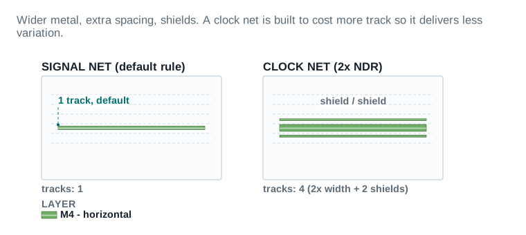
Signal net tracks consumed	1
Clock net tracks consumed (2x width + 2 shields)	4
Clock net capacitance vs signal (illustrative)	+34%

NDR on a clock net, worked Verified

Apply a 2x width rule to clk_core's root and internal nets before route_clock runs.

icc2_shell> set_clock_routing_rules -clocks [get_clocks clk_core] \
   -net_type internal -rules NDR_2X_CLOCK

2Confirm it is in force before routing, per Part 10's transition-violation symptom:
```
icc2_shell> clock_opt -to route_clock
```

Multibit optimization

Some libraries include multibit cells with mixed drive strength across their bits. If a violating path runs through a lower-drive-strength bit, the tool can rewire the cell so the path runs through a higher-drive-strength bit instead — enabled with clock_opt.flow.enable_multibit_rewiring. Separately, clock_opt.flow.enable_multibit_debanking allows the final_opto stage to split multibit registers apart when doing so improves timing and does not introduce hold violations.

Power or area recovery

If concurrent clock and data optimization is enabled — the default, and the subject of Part 7 — the tool performs clock power recovery on clock cells and registers during final_opto automatically. If CCD is disabled, you can still enable recovery explicitly with set_app_options -name clock_opt.flow.enable_clock_power_recovery -value power, or substitute -value area to recover area instead of power. Power recovery additionally requires scenarios enabled for power optimization via set_scenario_status's -dynamic_power and -leakage_power options, and optionally a switching activity file loaded with read_saif.

IR-drop-aware placement

During placement, the tool can use per-cell voltage-drop values to spread high-drop cells apart, reducing local power density. The recipe: run clock_opt -to route_clock, perform voltage-drop analysis with RedHawk Fusion's analyze_rail -voltage_drop static, enable place.coarse.ir_drop_aware, then finish with clock_opt -from final_opto.

Notice the shape of almost every advanced option in this Part: it is off by default, it requires a specific setup step before it does anything useful, and it changes the behaviour of a stage you would otherwise run identically every time. None of these are things you should reach for on a first pass through CTS. They exist for the second pass, when a specific number in a specific report tells you exactly which problem you are solving. Reaching for voltage-drop-aware synthesis before you have a voltage-drop problem is solving a problem you do not have yet, at the cost of runtime you do.

clock_opt runs build_clock, then route_clock, then final_opto, and each stage's output is a checkable, specific thing — built, routed, or legalized and globally routed. Run final_opto exactly once per block; every routing command after it assumes global routing already happened. The advanced options — voltage-drop awareness, NDR-aware optimization, multibit handling, power or area recovery, IR-drop-aware placement — are each solving one specific problem. Reach for them when you have that problem, not by default.

Part 7 — Concurrent clock and data optimization

The conceptual peak of the chapter

Everything before this Part treated the clock as something to balance as evenly as possible, then handed the result to the data path. Concurrent clock and data optimization — CCD — breaks that separation on purpose. It applies useful-skew techniques during data-path optimization, deliberately adjusting when the clock arrives at specific registers to take advantage of slack that already exists elsewhere on the path. By default, clock_opt performs CCD automatically; you disable it explicitly with clock_opt.flow.enable_ccd set to false if you do not want it.

Useful skew, in plain words

Say a path from FF1 to FF2 fails setup by 18 ps. The data path itself is fixed — CCD cannot touch logic. But the tool is allowed to delay the clock's arrival at FF2, the capture flop, by a controlled amount. Delay it 25 ps and the path now has 7 ps of positive slack. Nothing about the logic changed. What changed is when the clock told FF2 to capture.

Panel A: a path fails setup at -18 picoseconds. Panel B: the same path with capture delayed 25 picoseconds, now passing at +7 picoseconds. Panel C: the next path in the chain, whose margin shrank by 25 picoseconds to pay for it. — Read it: All three panels now draw FF1, FF2 and FF3 as real D flip-flop symbols, each with a visible CLK pin and edge-trigger triangle, name centred beneath its own body. Panel A: FF1 launches, FF2 captures, an arrow from FF1's Q pin into FF2's D pin, slack −18 ps, drawn in red. Panel B: same two flops, FF2's body now teal, a dimension arrow lands directly on FF2's CLK pin marking +25 ps added to its clock arrival, slack now +7 ps. Panel C, labelled THE COST: FF2 (still teal) now launches a second path to FF3, and that path's margin is called out as 25 ps thinner — the exact amount borrowed in panel B. Useful skew did not create margin. It moved it, and panel C shows where it came from.

Cost ledger — useful skew, drawn
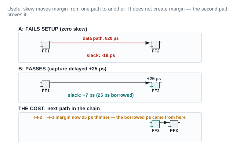
Path A before: slack	-18 ps
Path A after: capture delayed, slack	+7 ps (25 ps borrowed)
Path B (next in chain): margin lost	25 ps
Net margin created	0 ps — it moved, not grew

The reason Figure 11 draws a third panel is the single most important thing to understand about CCD, and it is easy to miss: useful skew never creates margin out of nothing. It borrows margin from wherever the register's other paths have slack to spare, and it pays that margin back by tightening whatever comes next. If you only look at the path you fixed, CCD looks like a free win. If you look at the whole chain, it is a trade, and a trade you should be able to explain, not just accept because the report says the target path now passes.

The controls: what you can limit

CCD's default behaviour touches every path in the block. Seven controls narrow that scope, all application options, all affecting place_opt, clock_opt, and route_opt alike unless noted:

Limiting the latency adjustment values. ccd.max_prepone bounds how far a clock can be advanced; ccd.max_postpone bounds how far it can be delayed. Neither has a default — you set both explicitly, in library timing units.
Excluding boundary paths. Set ccd.optimize_boundary_timing to false to exclude paths connected to boundary registers (transitive fanout of input ports, transitive fanin of output ports) from CCD. ccd.ignore_ports_for_boundary_identification lets you selectively keep specific ports' boundary paths in scope even with the exclusion on. A separate option, ccd.optimize_boundary_timing_upstream, controls whether the clock tree fanin of those excluded boundary registers can still change — leaving it at its default lets the tool optimize that fanin cone when doing so helps other, internal registers that share the same clock paths.
Excluding specific path groups. ccd.skip_path_groups takes a list of path group names, optionally scoped to a specific scenario.
Excluding specific scenarios. ccd.ignore_scenarios takes a list of scenario names to leave out of CCD entirely.
Excluding specific sinks. Set a cts_fixed_balance_pin attribute to true on the sink pin with set_attribute, then set ccd.respect_cts_fixed_balance_pins to true so the tool honors it. Setting that same option to upstream instead additionally prevents any change to the clock path between the fixed sink and the clock root.
Controlling timing optimization effort. ccd.timing_effort, low / medium (default) / high, affects the final_opt stage of clock_opt and route_opt.
Controlling hold optimization effort. ccd.hold_control_effort, default low, can be raised to medium, high, or ultra. Raising it trades away some setup-fixing capacity for more aggressive hold fixing — only raise it when hold is genuinely the critical constraint.

A separate, related control governs I/O clock latency adjustment specifically: by default the tool adjusts I/O clock latencies during CCD and again on any subsequent compute_clock_latency call. Disable it block-wide with ccd.adjust_io_clock_latency set to false, or scope it down to specific I/O clocks with set_latency_adjustment_options -exclude_clocks.

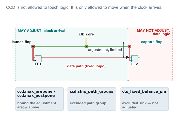
Figure 12 — CCD: what the tool is allowed to move A boundary diagram. Inside: clock arrival time at a sink, adjustable within limits. Outside: the data path's own logic, never adjustable. Three gate controls sit on the boundary: excluded path group, excluded scenario, excluded sink.

Read it: FF1 and FF2 are now real D flip-flop symbols, named beneath their own bodies. Left region, teal, MAY ADJUST: clock arrival time at a sink, bounded by ccd.max_prepone and ccd.max_postpone. Right region, red, MAY NOT ADJUST: the data path's own logic, cell selection, or connectivity — CCD never touches this. The two regions share a single boundary line, set just left of FF2's own CLK pin, so FF2's clock drop visibly crosses from teal into red exactly at the flop it is fixed by, with no overlap between the two shaded regions. Below both, three small boxes sit on the boundary between them: ccd.max_prepone / ccd.max_postpone, ccd.skip_path_groups, and cts_fixed_balance_pin, each labelled with what it excludes. CCD's entire toolkit lives inside the teal region; the boxes only ever narrow that region, never widen it into the red one.

Cost ledger — CCD: what the tool is allowed to move
Adjustable	clock arrival time at a sink
Not adjustable	data path logic and connectivity
Controls shown	3 (path group, scenario, sink exclusion)

Bound and scope CCD, worked Verified

Limit latency adjustment and exclude the boundary I/O paths, matching Dashboard 3's exclusions.

1Bound the adjustment:

icc2_shell> set_app_options -list {ccd.max_prepone 0.2}
icc2_shell> set_app_options -list {ccd.max_postpone 0.1}

2Exclude boundary paths except the two named I/O ports:

icc2_shell> set_app_options -name ccd.optimize_boundary_timing -value false
icc2_shell> set_app_options \
   -name ccd.ignore_ports_for_boundary_identification -value {IN_CLK OUT_CLK}

Dashboard 3 — CCD board

CCD moves margin; it never creates it. This board exists so a reviewer can see where the margin came from, not just that a path now passes.

CCD board — useful skew applied during final_opto
Item	Evidence	Source command / report	Threshold	Status	Required action
What moved
1. Sinks adjusted	14 of 4,210 clk_core sinks	`report_clock_timing -clock_crossing`	adjustments ≤ ccd.max_prepone/postpone	PASS	—
2. Paths improved	9 paths, setup slack now ≥ 0	`report_timing`	0 newly-failing paths introduced	PASS	—
3. Margin borrowed (sum, advanced sinks)	340 ps	ccd.max_prepone accounting	within configured budget	PASS	—
4. Margin given back (sum, delayed sinks)	340 ps	ccd.max_postpone accounting	balances against row 3 within rounding	PASS	—
Exclusions in force
5. Boundary paths excluded	ccd.optimize_boundary_timing = false, IN_CLK/OUT_CLK excepted	app-option review	matches the sign-off plan	PASS	—
6. Path groups excluded	0 — none excluded this run	`ccd.skip_path_groups`	matches the sign-off plan	PASS	—
7. Fixed-balance sinks respected	6 sinks, cts_fixed_balance_pin = true, 0 moved	`ccd.respect_cts_fixed_balance_pins`	0 of 6 moved	PASS	—

CCD verdict: 14 sinks adjusted, 9 paths improved, 0 paths made worse beyond -policy → accepted.

Read it: Row 3 and row 4 are a pair: 340 ps borrowed across 9 paths, 340 ps given back across the paths one hop further down the chain. If those two numbers do not roughly balance, CCD is being asked to create margin, not move it, and something upstream is wrong.

All figures are this chapter's illustrative teaching data.

Part 8 — Multisource clock trees

When you need one, and when you do not

The User Guide devotes about a third of its clock tree synthesis chapter to multisource structures. This Part is deliberately about a sixth of this one, because most readers of this guide will build a conventional clock tree many times before they ever need a multisource one. What follows is enough to recognize the structures, know when they earn their cost, and know where to go deeper if a real design demands it.

What a multisource clock tree is

A multisource clock tree is a custom clock structure built for more tolerance to on-chip variation and better cross-corner performance than a conventional tree achieves. It has two parts: a global clock structure — the root, a global clock tree usually shaped as an H-tree, clock mesh drivers, and the mesh itself — and local subtrees driven either by tap drivers connected to the mesh (a regular multisource clock tree, built with ordinary synthesize_clock_trees or clock_opt commands from those tap points) or directly from multiple points on the mesh, preserving a user-defined structure that is optimized by merging and splitting clock cells (a structural multisource clock tree).

The H-tree

An H-tree is a global clock structure shaped so every path from root to tap is geometrically equal by construction — the H shape repeats at each level, halving in size, so symmetry does the balancing work that buffer sizing would otherwise have to do.

Figure 13 — H-tree, drawn to scale on the Nimbus-8 core A symmetric H structure from the clock root at the core centre to four taps, equal path lengths, drawn on the 3.20 by 3.20 millimetre core outline.

Read it: The 3.20 x 3.20 mm core outline is drawn to scale. A horizontal spine crosses the centre; two vertical spines drop from its ends, each terminating at a tap. Every tap is now a real, named D flip-flop symbol — TAP1 through TAP4, symmetric around the centre root, each name printed directly beneath its own body. A dimension arrow labelled "L (equal, all 4 taps)" marks one root-to-tap path — the same length applies to all four by construction, which is the entire reason to build this shape instead of an ordinary fan-out tree.

Cost ledger — H-tree, drawn to scale
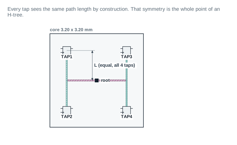
Taps	4
Path length to each tap	equal by construction
Levels	2
Core footprint used	3.20 x 3.20 mm (Nimbus-8 core)

Clock mesh

A clock mesh is the alternative global structure: a grid of shorted straps driven from multiple points, rather than a tree with distinct branches. Because every point on the mesh is electrically connected to every other point through the grid, local variation at any one driver gets averaged out across the whole structure — at the cost of the extra metal and extra power the grid itself consumes.

A grid of shorted straps on the same 3.20 by 3.20 millimetre core outline, drawn at the same scale as the H-tree so the two compare directly, with a note on the single simplified driver. — Read it: The same core outline, same scale as Figure 13. Three horizontal straps and three vertical straps cross to form nine shorted junctions across the grid. This figure simplifies the mesh to a single, centred driver for clarity; a real clock mesh is normally multisource, driven from several points at once — see “What a multisource clock tree is,” above. Compare the metal directly against Figure 13: the H-tree uses four discrete branches; the mesh uses a full grid across the same footprint. That difference in metal is the mesh's whole cost, and its whole benefit.

Cost ledger — clock mesh, same scale as Figure 13
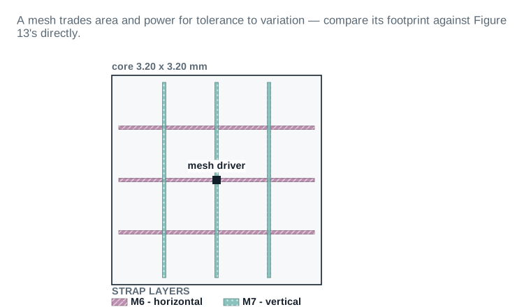
Strap rows / columns	3 / 3
Mesh drivers	1 (centre)
Footprint vs H-tree (Fig 13)	same core, more metal

“A mesh is always more robust, so it is always the safer choice.” A mesh is more tolerant of variation, but it is not free tolerance — compare the metal in Figure 14 against Figure 13 directly. That extra metal is extra capacitance, extra switching power, and extra routing resource consumed on layers your signal nets also want. Reach for a mesh when a real variation or skew problem on a conventional or H-tree structure cannot be solved any other way, not as a default because it sounds more robust.

Regular multisource, tap-driven, worked Verified

The shape of a regular multisource build, for a design that genuinely needs one — not run against Nimbus-8's four clocks in this chapter's worked example.

1Insert the tap drivers near their loads:

icc2_shell> create_clock_drivers -loads [get_pins tap_region1/*/CK] \
   -boxes {4 4} -lib_cells CKBUFX4

2Build the global clock tree structure:

icc2_shell> synthesize_multisource_global_clock_trees

3Check H-tree quality independently of the local subtrees:
```
icc2_shell> report_global_clock_tree_qor -type levelized
```

4Build the local subtrees from the tap drivers:

icc2_shell> synthesize_multisource_clock_subtrees

When you need one, and when you do not

A multisource structure earns its cost on very large, very high-frequency clock domains where a conventional tree's variation across the die becomes the dominant skew contributor, or where the floorplan itself makes a single balanced tree impractical — multiple disconnected regions of a hierarchical design, for instance. Nimbus‑8's clk_core at 1.60 GHz on a single partition, u_sens_tile, does not need one; a conventional tree with the exceptions Part 4 defined handles it. A design several times Nimbus‑8's size, at a higher frequency, spanning multiple partitions, would be the kind of design where this Part's structures stop being optional.

The commands behind multisource trees — synthesize_multisource_clock_subtrees, tap-driver insertion, clock strap creation, mesh analysis — are real and well documented, but they are also a commitment: once you build a structural multisource tree, the User Guide is explicit that subsequent ordinary clock tree synthesis commands will not change or remove it. You are choosing a different flow, not adding an option to the one you were already running. Make that choice deliberately, with a specific variation or floorplan problem in hand, not as an experiment.

Multisource clock trees — H-tree, clock mesh, structural subtrees built from tap drivers or mesh points — exist for large, high-frequency, or floorplan-constrained clock domains where a conventional tree's variation becomes the dominant problem. They cost real metal, area and power, visible directly by comparing Figures 13 and 14. Most designs, including Nimbus‑8's four clocks, do not need one. Know the structures well enough to recognize when a real design does.

Part 9 — Reading the reports

Where knowledge turns into competence

You can know every term from Part 2 and every command from Parts 4 through 7 and still not be able to read a real QoR report cold. This Part closes that gap. It is organized around one command, report_clock_qor, and it teaches you to read its output line by line, in the order that actually matters, not the order the report happens to print them in.

report_clock_qor: what it can show you

By default, report_clock_qor prints a summary — latency, skew, DRC violations, area, and buffer count. Beyond the default summary, the -type option unlocks several specific views: latency for the longest and shortest path per clock, drc_violators for maximum-transition and maximum-capacitance violators, robustness for how a sink's latency in the reported corner compares to a named robustness corner, balance_groups for a per-skew-group summary, local_skew for the worst local skew per clock or group along with the five largest and five smallest values and their endpoints, and power for a leakage/internal/sink/net-switching/dynamic/total power breakdown per clock per scenario. Add -csv summary or -csv details with -output to export any of these to a file instead of the shell. The command can also produce histograms — latency, transition, capacitance, local skew, robustness, and wire-delay fraction — through -histogram_type.

An annotated report_clock_qor summary block for clk_core, with callouts marking the read order: latency first, global skew second, local skew third, violator counts checked before trusting any of it. — Read it: A dark report panel lists clk_core's summary fields: latency 118/154 ps, global skew 36 ps, local skew 9 ps, buffer count 38, and two violator counts, both 0. Four callouts on the right, each leader landing level with the row it names: "read first: latency" points at the latency row, "read second: headline skew" points at global skew, "read third: closes timing" points at local skew, and "check before trusting: 0 violators" points at the two violator lines at the bottom. The read order is deliberate — it is not the order the fields are printed in.

Cost ledger — reading a clock QoR report
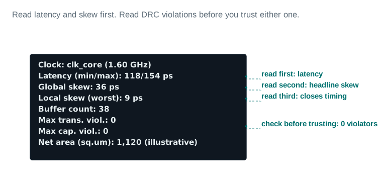
Fields called out	4 (latency, global skew, local skew, DRC)
Fields in the raw report	8
Read order taught	latency → global skew → local skew → DRC

Read latency first because it tells you how many levels the tree is running, which sets your expectations for every other number. Read global skew second as a smoke-detector check on overall tree health. Read local skew third, because it is the number that actually decides pass or fail on a real path. And check the violator counts before you trust any of the first three — a tree with excellent skew and latency numbers but active transition violations on clock nets is not actually a good tree; the violations mean the numbers you are reading may not survive signoff extraction.

Dashboard 4 — post-build QoR board

This is the board that turns a finished build_clock run into a go/no-go for route_clock. Two columns decide it: skew and violations.

Post-build QoR board — per clock, after build_clock
Item	Evidence	Source command / report	Threshold	Status	Required action
Skew and latency
1. clk_core: global / local skew	36 ps / 9 ps	`report_clock_qor -type local_skew`	≤ 40 ps global / ≤ 15 ps local	PASS	—
2. clk_dsp: global / local skew	48 ps / 12 ps	`report_clock_qor -type local_skew`	≤ 55 ps global / ≤ 18 ps local	PASS	—
3. clk_io: global / local skew	61 ps / 14 ps	`report_clock_qor -type local_skew`	≤ 70 ps global / ≤ 20 ps local	PASS	—
4. clk_pwr: global / local skew	77 ps / 19 ps	`report_clock_qor -type local_skew`	≤ 90 ps global / ≤ 25 ps local	PASS	—
Structure and violations
5. clk_core: levels / buffers / insertion delay	4 levels, 38 buffers, 118-154 ps	`report_clock_qor -type latency`	insertion delay ≤ 180 ps	PASS	—
6. clk_dsp: levels / buffers / insertion delay	4 levels, 31 buffers, 142-190 ps	`report_clock_qor -type latency`	insertion delay ≤ 220 ps	PASS	—
7. Transition violators, all clocks	0	`report_clock_qor -type drc_violators`	0 violators	PASS	—
8. Capacitance violators, all clocks	0	`report_clock_qor -type drc_violators`	0 violators	PASS	—

QoR verdict: 4 of 4 clocks inside target skew, 0 transition/capacitance violators → proceed to route_clock.

Read it: Read the local-skew column, not the global-skew column, if you only have time for one: clk_core's local skew (9 ps) is the number Figure 17E measures at the end of this chapter's worked example.

Latency, skew and buffer counts are this chapter's illustrative teaching data.

Clock tree power

Use report_clock_qor -type power for the leakage, internal, sink, net-switching, dynamic, and total power breakdown per clock per scenario. If power.clock_network_include_clock_sink_pin_power is set to off, sink power is excluded from the total — worth confirming before comparing power numbers across two different report runs, since a mismatched setting will make two runs look inconsistent when they are not.

Dashboard 5 — clock power and area board

A clock tree that closes timing but blows the power budget is not done. This board is where that gets caught.

Clock power and area board — what the tree costs
Item	Evidence	Source command / report	Threshold	Status	Required action
Cell count and area
1. Clock cell count, all 4 trees	146 buffers/inverters	`report_clock_qor -type summary`	tracked against budget of 180	PASS	—
2. Clock cell area, all 4 trees	1,120 sq.um	`report_clock_qor -type summary`	≤ 0.02% of core area	PASS	—
3. Clock net length, all 4 trees	18.4 mm total	clock net length report	tracked, no hard threshold	PASS	—
Power
4. Clock switching power / total dynamic power	9.4% (2.1 mW of 22.3 mW)	`report_clock_qor -type power`	≤ 12% of total dynamic power	PASS	—
5. Power recovered by final_opto	0.3 mW, 4 buffers removed, 0 skew/latency regression	`clock_opt.flow.enable_clock_power_recovery`	recovery attempted, no QoR regression	PASS	—
6. Clock leakage power share	0.6% of total leakage	`report_clock_qor -type power`	tracked, no hard threshold	PASS	—

Power/area verdict: clock network 9.4% of total dynamic power, within the 12% budget → within budget.

Read it: Row 5 is the one worth a second look: area recovery removed 4 buffers with no skew or latency regression, which is the clock_opt.flow.enable_clock_power_recovery pass Part 6 describes.

All figures are this chapter's illustrative teaching data.

Local skew and latency reports, worked Verified

Two calls that back Dashboard 4's row 1 and row 5 for clk_core.

1Local skew, per clock:

icc2_shell> report_clock_qor -clocks [get_clocks clk_core] -type local_skew

2Longest and shortest path latency:

icc2_shell> report_clock_qor -clocks [get_clocks clk_core] -type latency

Analyzing clock timing

report_clock_timing reports the timing attributes of clock networks directly — per clock, per mode, per corner, per scenario, with options to scope by setup or hold, launch or capture, rise or fall, and to report clock crossings and physical detail. Use it when a specific path's clock-side timing, not the tree's aggregate QoR, is the question — for instance, tracing exactly how much latency adjustment CCD applied at one specific sink, the same accounting Dashboard 3 in Part 7 summarizes at the tree level.

Collections of clock network pins

Beyond the report commands, you will often need a raw collection of clock network objects — every sink pin on clk_core, every ignore pin across all four clocks — to feed into a script or a custom check. get_pins combined with the is_clock_is_used_as_clock attribute from Part 4, or report_clock_balance_points for exception-specific collections, are the tools for that, and they are worth knowing exist even before you need them for something specific.

Part 10 — Troubleshooting by symptom

Start from what you see, not from what the tool calls it

A beginner staring at a bad QoR report does not think in tool vocabulary yet. They see a symptom: skew missed the target, or a hold violation showed up out of nowhere. This Part is organized by symptom, not by tool terminology, because that is how the problem actually reaches you the first time.

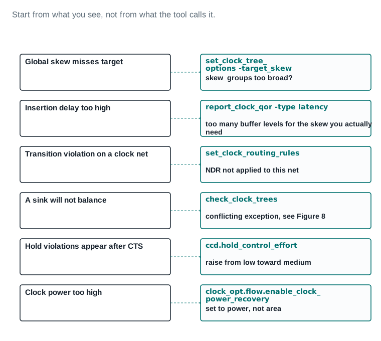
Six symptom boxes, each connected to a leaf naming the command, the likely cause, and the setting to check: skew miss, latency too high, transition violation, unbalanced sink, post-CTS hold, and power too high. — Read it: Six rows, each a symptom box on the left connected by a dashed leader to a teal command box on the right. Global skew misses target leads to `set_clock_tree_options -target_skew`, checking whether skew groups are too broad. Insertion delay too high leads to `report_clock_qor -type latency`. Transition violation leads to `set_clock_routing_rules`, checking whether the NDR was applied. Unbalanced sink leads to `check_clock_trees`, pointing back at Figure 8's balancing conflict. Post-CTS hold leads to `ccd.hold_control_effort`. Power too high leads to `clock_opt.flow.enable_clock_power_recovery`, checking whether it is set to power rather than area.

Cost ledger — troubleshooting decision tree
Symptoms covered	6
Commands referenced	6, each verified in the body

Symptom: global skew misses target

Likely cause: skew groups are too broad, forcing sinks that do not need to match each other into the same balancing target, or a target-skew value that does not match what the tree's actual structure can achieve. What to check: report_clock_qor -type balance_groups to see per-group targets against actuals. What to change: narrow skew groups around sinks that genuinely share timing paths, per Part 5, before assuming the target itself is unreachable.

Symptom: insertion delay too high

Likely cause: too many buffer levels for the skew you actually need — Part 2's Figure 3 lesson, showing up as a real number instead of an illustration. What to check: report_clock_qor -type latency for the level count and per-level contribution. What to change: loosen the target skew slightly if the current target is forcing more levels than the design needs, rather than accepting whatever latency the tool needed to hit an unnecessarily tight target.

Symptom: transition violation on a clock net

Likely cause: a non-default routing rule was not actually applied to the net carrying the violation, or the rule was applied after route_clock already ran. What to check: set_clock_routing_rules settings against the specific net, and confirm the rule was in place before routing, not after. What to change: apply the NDR and rerun route_clock; an NDR set after routing has no effect on already-drawn metal.

Symptom: a sink will not balance

Likely cause: a balancing conflict — the sink sits behind a macro or in a different voltage area, exactly Figure 8's picture. What to check: check_clock_trees for reported balancing conflicts on that sink. What to change: either accept the conflict and mark the sink an ignore pin deliberately, per Part 4, or, if balancing genuinely matters for that sink, reconsider the floorplan decision that created the conflict in the first place.

Symptom: hold violations appear after CTS

Likely cause: real clock latency, once the tree is built, shifted the effective timing window enough to expose a hold margin that the ideal-clock assumption before CTS was hiding. What to check: whether the violations are new, or were always marginal and just crossed the line once real clock skew replaced uncertainty. What to change: raise ccd.hold_control_effort from low toward medium if the violations are widespread; for isolated cases, a targeted hold fix downstream of CTS is often cheaper than reworking the tree.

Notice that every "what to check" column in this table names a report or a settings query, never a guess. The difference between a beginner and an experienced engineer debugging the same symptom is rarely knowledge of more commands — it is the discipline to run the check before changing a setting. Changing target_skew because a tree looks unbalanced, without first reading report_clock_qor -type balance_groups to see whether the target itself is achievable, wastes a run. Check first. Change second.

Diagnose a transition violation, worked Verified

Confirm the violator, confirm the rule, then re-route.

1List the violators:

icc2_shell> report_clock_qor -clocks [get_clocks clk_core] -type drc_violators

2Confirm whether an NDR is actually in force on the violating net before assuming it is missing:
```
icc2_shell> report_clock_settings -clocks [get_clocks clk_core]
```

Symptom: clock power too high

Likely cause: power recovery during final_opto was not enabled, or was set to recover area instead of power. What to check: clock_opt.flow.enable_clock_power_recovery's current value. What to change: set it explicitly to power rather than area if power is the binding constraint, and confirm scenarios are enabled for dynamic and leakage power optimization first — recovery cannot run without that prerequisite.

Part 11 — Worked example and guided lab

clk_core, end to end, on Nimbus-8

Every concept in this chapter now comes together on one tree: clk_core, the 1.60 GHz clock rooted in u_sens_tile, the hardest of Nimbus-8's four clocks. Five panels, one locked coordinate frame — the same region, the same macro, the same pixel positions in every panel, so you can watch the tree accumulate state without your eye having to re-orient each time. A five-column status strip runs beneath every panel: defined, exceptions, built, routed, skew. A field not yet decided shows a dash.

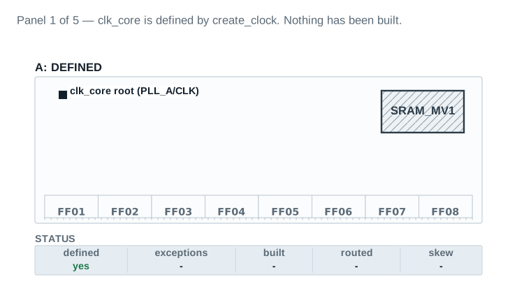
u_sens_tile region, root marked with a navy square, clocks defined, no tree yet. — Read it: The region shows SRAM_MV1 in the upper right and eight named flops, FF01 through FF08, in a row along the bottom. A navy square marks the root, labelled clk_core root (PLL_A/CLK). No wires connect anything yet. Status strip: defined yes, exceptions dash, built dash, routed dash, skew dash.

Cost ledger — 17A: defined
Clock defined	clk_core, 1.60 GHz
Exceptions / built / routed / skew	- / - / - / -

create_clock -name clk_core -period 0.625 [get_pins PLL_A/CLK] is the single line of SDC that puts this panel's one fact on the board. Nothing physical exists yet — this is the ideal-clock world Part 1 described, captured at the instant before it starts to change.

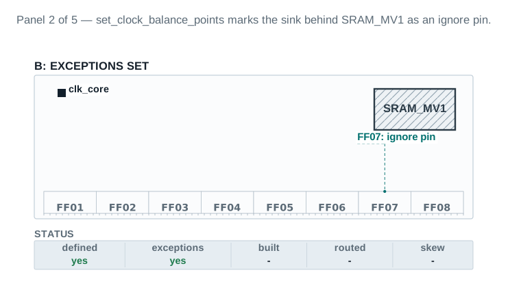
Same region, FF07 marked as an ignore pin behind SRAM_MV1. — Read it: Identical geometry to 17A. A leader line now points from below the cell row up toward SRAM_MV1's position, labelled "FF07: ignore pin." Status strip: defined yes, exceptions yes, built dash, routed dash, skew dash.

Cost ledger — 17B: exceptions set
Ignore pins set	1 (FF07)
Command	set_clock_balance_points -consider_for_balancing false

FF07 sits behind SRAM_MV1, in a separate voltage area — Figure 8's conflict, now applied to the real worked tree. set_clock_balance_points -clock [get_clocks clk_core] -consider_for_balancing false -balance_points [get_pins u_sens_tile/FF07/CLK] marks it as an ignore pin: excluded from balancing, still reached, still DRC-fixed.

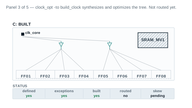
Same region, two level-1 buffers placed, thin dashed guide lines to each sink, unrouted. — Read it: Two teal buffer triangles now sit between the root and the cell row — level-1 buffers, drawn as the same schematic symbol used everywhere else in this chapter. Dashed lines, not filled metal, connect root to buffers and buffers to each of the eight sinks below; SRAM_MV1 sits clear of the tree, top right, drawn as a plain blockage outline with no dangling pin stubs. Status strip: defined yes, exceptions yes, built yes, routed no, skew pending.

Cost ledger — 17C: built
Buffers placed	2 (level 1, this region)
Routed	no — guide lines only

clock_opt -to build_clock produces exactly this state: the tree is synthesized and optimized logically, and the clocks are now propagated, but nothing is routed. The dashed lines are a deliberate visual choice — they are guide connections, not metal, and drawing them any other way would misrepresent what build_clock actually produces.

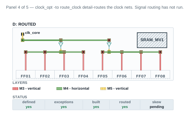
Same region, the tree now real filled metal on M3 through M5, with a layer legend. — Read it: The same two buffers and eight sinks, now connected by solid filled metal — M5 from root to buffers, M4 and M3 down to the sinks, wider than a default-rule signal net per Part 6's NDR discussion, each via drawn once at its real junction. A layer legend below names all three. SRAM_MV1, top right, stays clear of every trunk and drop with visible margin. Status strip: defined yes, exceptions yes, built yes, routed yes, skew pending.

Cost ledger — 17D: routed
Layers used	M3, M4, M5
Trunk width	2x default (NDR)

clock_opt -from route_clock -to route_clock detail-routes exactly these nets, using the NDR set in Part 5. Skew is still marked pending: it was estimated during build_clock, but the number that matters is the one measured against real, routed parasitics, and that number does not exist until the next panel.

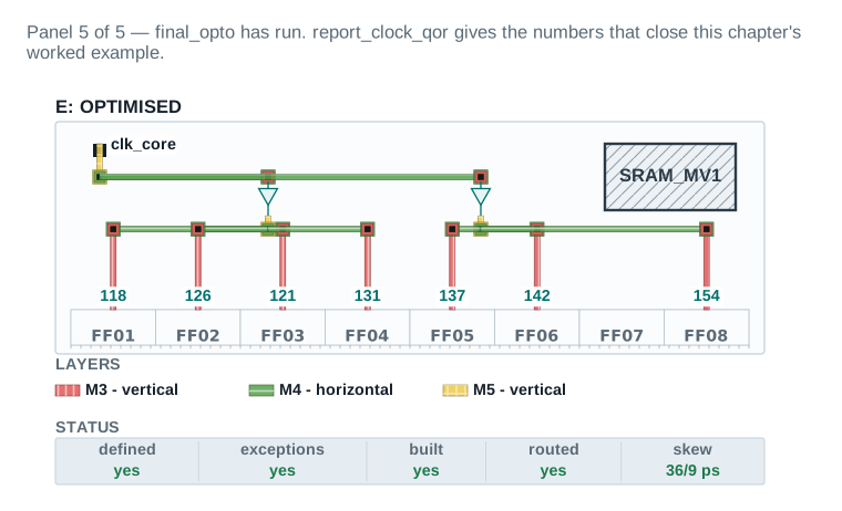
Same region, arrival times annotated on each of the seven balanced sinks, global skew 36 picoseconds, local skew 9 picoseconds. — Read it: Identical geometry to 17D, including its layer legend below the panel — the seven red M3 sink drops are metal, keyed there, not a violation marker. Each of the seven balanced sinks (FF07, the ignore pin, is skipped) now carries a small arrival-time annotation in teal. Status strip: defined yes, exceptions yes, built yes, routed yes, skew 36/9 ps — global over local, the same pairing Figure 2 taught in Part 2.

Cost ledger — 17E: optimised and measured
Global skew	36 ps
Local skew, worst pair	9 ps
Sinks measured	7 of 8 (FF07 is the ignore pin, not balanced)

clock_opt -from final_opto completes the flow: optimization, legalization, and global routing against real, routed parasitics. report_clock_qor -clocks clk_core now returns the numbers this chapter has been building toward — 36 ps global skew, 9 ps local skew on the worst pair, the same figures Dashboard 4 records in Part 9.

clk_core, all five stages, worked Verified

Every command behind Figures 17A through 17E, in order.

1Define (17A):

icc2_shell> create_clock -name clk_core -period 0.625 [get_pins PLL_A/CLK]

2Set exceptions (17B):

icc2_shell> set_clock_balance_points -clock [get_clocks clk_core] \
   -consider_for_balancing false -balance_points [get_pins u_sens_tile/FF07/CLK]

3Build (17C):
```
icc2_shell> clock_opt -to build_clock
```

4Route (17D):

icc2_shell> clock_opt -from route_clock -to route_clock

5Optimize and measure (17E):

icc2_shell> clock_opt -from final_opto
icc2_shell> report_clock_qor -clocks [get_clocks clk_core]

Guided lab: repeat it for clk_dsp

Run the same five-stage sequence — define, set exceptions, build, route, optimize and measure — against clk_dsp, the 1.10 GHz clock on u_dsp_core. Its five ignore pins and its own balancing conflicts are different from clk_core's single one, which is deliberately the point: the mechanics are identical, the specific exceptions are not, and a lab that only ever touches one clock never tests whether you understood the mechanics or just memorized one example's numbers.

A locked coordinate frame across five panels is not a stylistic choice — it is how you prove to yourself, and to anyone reviewing your work, that nothing silently moved between stages except what the stage's own command is supposed to change. If a cell drawn in panel C is missing from panel D with no explanation, that is a real defect, not a drawing inconsistency, and the same discipline applies to a real design: every stage of clock_opt should account for every cell it started with.

Part 12 — Stage exit and handoff to routing

What leaves this stage, and what routing must not touch

This Part closes the chapter's third question — how do I prove the tree is real — with a single gate. Everything CTS produced either passes this gate or it is not ready to hand off, no matter how good any individual number looked along the way.

What leaves CTS

Propagated clocks. Every clock in the design, not just clk_core, must be propagated — the ideal-clock fiction from Part 1 must be gone everywhere, not just in the tree you happened to worked-example through.
A routed clock network. 100% of clock nets detail-routed, on the NDRs Part 5 defined, verified against real metal, not an estimate.
A QoR report, archived. report_clock_qor output, per clock, saved alongside the design — not just glanced at in a shell session and discarded.
Both scenarios timed. func_ss_0p72v_125c for setup and func_ff_0p88v_m40c for hold, both closed, not just the one scenario that happened to be active when you last ran clock_opt.

Figure 18 — What leaves this stage A handoff card listing five gates, all passing, and one instruction to routing: do not disturb the clock network.

Read it: Five checklist rows, each with a green square and a short statement: clocks propagated, clock network fully routed, QoR report archived, both scenarios timed, zero transition/capacitance violations on clock nets. Below the list, an amber box states the one instruction routing inherits: a clock network it must not disturb — route_opt and ECO flows must not rip up clock routing.

Cost ledger — what leaves this stage
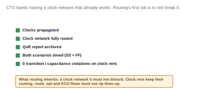
Gates checked	5
Gates passing	5 of 5
Instruction to routing	do not disturb the clock network

Dashboard 6 — stage exit go/no-go

This is the last board in the chapter. Every row here is something routing will assume is already true and will not re-check.

Stage exit go/no-go — ready to hand off to routing?
Item	Evidence	Source command / report	Threshold	Status	Required action
Clocks and network
1. All 4 clocks propagated	4 of 4	`synthesize_clock_trees -propagate_only` status	4 of 4 propagated	PASS	—
2. Clock network fully routed	100% of clock nets	`clock_opt -to route_clock` status	100% routed	PASS	—
3. Skew within target, all 4 clocks	4 of 4	Dashboard 3	4 of 4 within target	PASS	—
4. Insertion delay within target, all 4 clocks	4 of 4	Dashboard 3	4 of 4 within target	PASS	—
Signoff and archive
5. Both scenarios timed	func_ss_0p72v_125c and func_ff_0p88v_m40c	`report_timing`	both scenarios present	PASS	—
6. 0 transition violations, clock nets	0	`report_clock_qor -type drc_violators`	0 violations	PASS	—
7. 0 capacitance violations, clock nets	0	`report_clock_qor -type drc_violators`	0 violations	PASS	—
8. QoR report archived	clk_core_qor_final.rpt and 3 others, stored	`report_clock_qor -csv summary -output`	archived alongside the ECO record	PASS	—
9. Checkpoint saved and reopens	`nimbus8_sens_tile_cts_closed_v1`	`save_block` / reopen test	exists, reopens with 0 errors	PASS	—
10. Handoff note to routing written	"do not disturb the clock network" recorded	Part 12 close	present	PASS	—

Exit verdict: 10 of 10 PASS → GO — handoff to routing approved.

Read it: Read row 9 last, not first: the checkpoint is the artifact routing actually opens. Everything above it is what makes that checkpoint trustworthy.

Field values are this chapter's illustrative teaching data.

Propagate remaining scenarios and archive, worked Verified

Dashboard 6, rows 1 and 9, produced.

1Propagate any scenario activated after the main build:
```
icc2_shell> synthesize_clock_trees -propagate_only
```

2Archive the QoR report:

icc2_shell> report_clock_qor -csv summary -output clk_core_qor_final.rpt

3Save the checkpoint:

icc2_shell> save_block -as nimbus8_sens_tile_cts_closed_v1

The handoff to routing

Routing inherits a clock network that already works. Its first job, before it routes a single signal net, is to not break that network. final_opto already global-routed every signal net as part of its own last step, which is exactly why the User Guide is emphatic that final_opto runs once per block: everything downstream of it assumes the global route picture it produced is still accurate. A detail router that reroutes clock nets, or a change to routing setup after clock_opt completed, breaks that assumption directly.

“Routing can adjust the clock nets a little if it helps congestion.” It should not, and the tools are built around the expectation that it will not. Clock nets carry design-rule-clean, skew-verified, power-budgeted routing that every number in this chapter's dashboards was measured against. A routing pass that quietly reroutes even one clock segment invalidates the skew and timing numbers CTS signed off, silently, with no warning that anything changed. If congestion genuinely requires touching clock routing, that is a CTS decision to revisit — new NDRs, a different tree structure — not a routing-stage adjustment.

Every stage-exit gate in this series has the same shape: a short list of facts the next chapter is allowed to assume without re-checking. That is what makes an eight-chapter flow tractable at all — Chapter 6 does not re-verify that your clocks are propagated any more than this chapter re-verified that Chapter 4's placement was legal beyond the one prerequisite check in Part 3. Each stage trusts the previous stage's gate. That trust is only warranted if the gate was actually checked, with real numbers, not assumed because the last few runs happened to look fine.

Part 13 — Knowledge reinforcement and interview bank

45 questions, tiered, every answer grounded in this chapter

Forty-five questions across four tiers: 16 beginner, 15 intermediate, 9 advanced, and 5 senior/architect (16+15+9+5 = 45). Every answer draws only on what this chapter taught; illustrative numbers are labelled as such, and no command appears in an answer that was not verified in the body text. At least six questions cross back to other chapters, marked ↩ other chapter.

Beginner, 16 questions

1. What is skew?: The difference in arrival time between two points on a clock network. Global skew is the spread across every sink in a group; local skew is the difference between two sinks that share a real timing path.
2. What does "propagated" mean, for a clock?: A clock is propagated once its real, physical insertion delay and skew replace the zero-delay, arrives-everywhere-at-once assumption used before CTS. build_clock sets synthesized clocks as propagated as soon as it completes.
3. What is an ignore pin?: A pin explicitly excluded from balancing with set_clock_balance_points -consider_for_balancing false. It is still reached by the tree, and any design-rule violations on the branch beyond it are still fixed during optimization.
4. What are the three stages of clock_opt?: build_clock, route_clock, and final_opto, run in that order by default.
5. What is insertion delay?: The time it takes the clock to travel from its root to a given sink, also called latency. It is not free, and lowering skew by adding buffer levels always raises it.
6. Which command checks that clock trees are correctly defined?: check_clock_trees. Called with -clocks, it scopes to a list; without it, it checks every clock in the block.
7. What command sets an insertion delay override on a sink pin?: set_clock_balance_points, using its -delay option, with -rise/-fall/-early/-late to scope which calculations it applies to.
8. What are the four hard prerequisites before CTS?: Legal placement, correctly defined clocks, prerouted power and ground, and the right active scenarios enabled. Legal placement is not re-derived here — it is the same legality check Placement and Optimization already established. ↩ Placement and Optimization
9. What does clock uncertainty represent, before CTS runs?: A conservative placeholder margin for skew that has not been built yet. Once CTS produces a real, measured skew number, some of that margin is returned to the data paths.
10. What is a clock-gating cell's enable path?: A separate timing path into the ICG's enable input, with its own timing check independent of the clock path itself — it must be stable before the clock edge it gates.
11. Which command reports clock tree quality of results?: report_clock_qor. Its default view is a summary of latency, skew, DRC violations, area and buffer count; -type unlocks more specific views.
12. What is a skew group?: A named subset of a clock's sinks balanced against each other and reported on separately, set with set_clock_tree_options -skew_groups.
13. What is the H-tree structure used for?: A global clock structure, usually part of a multisource clock tree, shaped so every root-to-tap path is geometrically equal by construction — symmetry does the balancing work.
14. Which application option enables CCD, and is it on by default?: clock_opt.flow.enable_ccd. It is enabled by default; set it to false to disable concurrent clock and data optimization.
15. What does report_clock_qor -type drc_violators show?: Maximum-transition and maximum-capacitance constraint violators on the clock network.
16. What must run exactly once per block, and why?: final_opto. After it completes, every signal net is global routed, and subsequent routing commands skip global routing on that assumption — running it again or changing routing setup afterward breaks that assumption.

Intermediate, 15 questions

17. Why is local skew the number that actually closes timing, not global skew?: Local skew measures the arrival-time difference between two sinks that share a real timing path — the launch and capture flops on a specific path. That is what determines pass or fail on that path. Global skew is the spread across every sink, including pairs that never appear together on any real path, so it can look bad while every actual path closes, or look good while one bad local pair fails.
18. Why does final_opto run timing-driven placement and a full global route, not just optimization?: Because it is optimizing against real, routed clock parasitics for the first time in the flow, the design's placement and routing may both need adjustment to close timing against that new reality — not just cell sizing. Running a full global route at this stage also gives every subsequent routing command an accurate picture to build on.
19. What does a balancing conflict look like, and what typically causes one?: A sink the tool cannot balance against its siblings without violating some other constraint — typically because it sits behind a hard macro, in a separate voltage area, or on a path handled by another mechanism entirely. Figure 8 draws exactly this: a sink physically blocked from a direct, comparable path to the root, in a position the floorplan committed to before CTS ever ran. ↩ Floorplan
20. Why does clock uncertainty shrink after CTS runs?: Because uncertainty before CTS is a conservative estimate standing in for skew that has not been measured yet. Once CTS produces a real skew number, that number replaces the estimate in timing analysis, and because the estimate was conservative, the replacement is usually smaller — the difference is margin returned to the data paths.
21. What happens if you set a clock tree exception on a pin whose is_clock_is_used_as_clock attribute is false?: The command is accepted without error, but the tool ignores the exception during clock tree synthesis, because it has already classified that pin as part of the data network rather than the clock network. This is a silent failure mode — always re-verify exceptions with check_clock_trees.
22. Why does useful skew always show up as a cost somewhere else, not just a benefit on the target path?: Because CCD cannot create timing margin — it can only move clock arrival time at a sink, which borrows slack from wherever that sink's other paths have margin to spare, and gives it to the target path. Whatever path shares that sink's clock edge downstream now has less margin than it had before.
23. What is the difference between ccd.optimize_boundary_timing and ccd.optimize_boundary_timing_upstream?: The first excludes boundary-register paths themselves from CCD. The second, independently, controls whether the clock tree fanin cone feeding those excluded boundary registers can still change to help other, internal registers on shared clock paths — turning it off heavily restricts CCD's scope beyond what the first option alone does.
24. Why is target_latency's default different from target_skew's default?: Target skew defaults to 0, which the tool interprets as "minimize skew" rather than a literal requirement. Target latency has no default at all — you only set it when you specifically need a minimum early insertion delay floor, which is not a universal requirement the way some amount of skew minimization is.
25. Why must NDRs on clock nets be set before route_clock, not after?: Non-default routing rules only affect metal that has not been drawn yet. route_clock detail-routes the clock nets using whatever rules are in force at that moment; applying an NDR afterward has no effect on already-routed geometry and requires a re-route to take effect.
26. What does the robustness metric in report_clock_qor actually measure?: The ratio between a sink's latency in the reported corner and its latency in a separately specified robustness corner, for the same mode. It is a cross-corner consistency check, not a skew or latency value in isolation.
27. Why does power recovery require scenarios enabled for dynamic or leakage power optimization first?: Because clock_opt.flow.enable_clock_power_recovery operates during power-aware optimization passes that only run when the active scenarios are explicitly told, via set_scenario_status -dynamic_power or -leakage_power, that power is a metric to optimize for — without that, the recovery pass has nothing to act on.
28. Why does hold_control_effort default to low rather than medium?: Because raising hold-fixing effort reduces the number of setup violations CCD fixes — effort spent on hold is effort not spent on setup. The low default reflects that most designs are setup-critical more often than hold-critical during CCD, and raising it should be a deliberate choice made because hold is genuinely the binding constraint, not a default.
29. What is the practical difference between a regular and a structural multisource clock tree?: A regular multisource tree's local subtrees are built with ordinary synthesize_clock_trees or clock_opt commands from tap-driver points on the mesh. A structural multisource tree instead preserves a user-defined structure, optimized by merging and splitting clock cells, and once built, ordinary CTS commands will not change or remove it — it is a distinct, committed flow.
30. Why is post-CTS hold analysis often different from pre-CTS hold analysis, even with no logic changes?: Pre-CTS hold analysis uses an ideal, often zero-skew clock, which tends to be optimistic about hold margin. Real, unequal arrival times from the built tree replace that assumption, and paths that were always marginal on hold simply become visible once the real numbers are in place — not because anything about the logic changed.
31. Why should a mesh's extra cost be weighed against an H-tree's, not assumed automatically justified?: A clock mesh's tolerance to variation comes from extra shorted metal across the whole structure, visible directly by comparing Figures 13 and 14 at the same scale. That metal is real capacitance, real switching power, and real routing resource taken from layers signal nets also want. It earns its cost only when a real variation problem a simpler structure cannot solve is actually present.

Advanced, 9 questions

32. When do you accept higher insertion delay to get lower skew?: When the design's actual timing margin cannot absorb the skew a shallower tree produces, and the added latency the deeper tree costs still leaves enough room on the critical paths after accounting for the extra on-chip-variation exposure the added levels bring. Accepting it without checking the latency budget against real paths is how a tree ends up "balanced" and still failing timing on latency-sensitive paths.
33. When is useful skew the right tool, and when is it borrowing you cannot repay?: It is the right tool when the path receiving the borrowed margin has genuine slack to spare and the path paying for it still closes with room left. It is borrowing you cannot repay when CCD is asked to fix a path whose neighbors are all already tight — in that case the "fix" just relocates the failure to a path that was not failing before, and the aggregate timing has not actually improved.
34. When do you need a multisource tree rather than a conventional one?: When a conventional tree's cross-die variation becomes the dominant contributor to skew that cannot be solved by adjusting skew groups or buffer levels, typically on very large or very high-frequency domains, or when the floorplan itself — multiple disconnected regions of a hierarchical design — makes a single balanced tree impractical to build at all.
35. Why exclude a path group from CCD rather than letting it optimize freely?: Because some path groups carry timing relationships CCD's general-purpose borrowing logic should not touch — a group with an external interface timing contract, for instance, where clock arrival at the boundary is fixed by something outside the block's control. ccd.skip_path_groups protects that contract explicitly rather than trusting CCD to infer it should leave the group alone.
36. Why does the tool distinguish -clock_path from -data_path on set_max_transition and set_max_capacitance?: Because clock nets and data nets have different tolerances for transition degradation and different loading profiles — a clock net typically drives many loads and any edge degradation compounds across the whole tree, so scoping the limit specifically to the clock path lets you set a tighter rule there without over-constraining every data net in the design.
37. Why is nworst skew optimization needed, given the tool already optimizes global skew directly?: The multithreaded clock tree optimization engine minimizes the delay difference between the longest and shortest paths by default, and if optimization stalls on the shortest path, the remaining paths can stay under-optimized. Enabling cts.optimize.enable_nworst_skew_optimization optimizes across the n worst paths instead of bailing out early on just the extremes, avoiding that stall.
38. Why does the User Guide caution against changing global route shapes after clock_opt completes?: Because final_opto's last action is a full global route of every signal net, and every subsequent routing command — route_auto, route_global, route_group — checks whether global routing already happened and skips it if so. A change to global route shapes after that point creates a mismatch between what the router believes is true and what actually is, which surfaces as track-assignment or detail-routing errors.
39. How would you decide between raising ccd.hold_control_effort and fixing hold violations downstream of CTS by hand?: Raise the effort level when hold violations are widespread across the design, because it is a single setting that improves the whole picture at once, at the cost of some setup-fixing capacity. Fix violations by hand, downstream, when they are isolated to a handful of paths, because a targeted fix does not cost setup margin everywhere else the way a block-wide effort increase does.
40. Why can a tree with excellent skew and latency numbers still be a bad tree?: Because those numbers alone say nothing about design-rule health, power, or robustness across corners. A tree with tight skew and short latency but active transition violations on its clock nets, or power well outside budget, or poor robustness in a corner the signoff numbers were not measured against, has not actually proven itself — the full QoR picture, not two favorable numbers, is what decides whether a tree is good.

Senior / architect, 5 questions

41. How do you budget clock power against a chip-level target?: Start from the chip-level dynamic power budget and allocate a share to the clock network based on frequency and fanout — Nimbus‑8's own clock network runs close to a tenth of total dynamic power, tracked explicitly in Dashboard 5. Measure actual clock power per clock with report_clock_qor -type power after every major CTS run, not just once at the end, so a budget overrun is caught while there is still time to enable power recovery or revisit tree structure, rather than discovered at the final signoff power check. ↩ Chip Finishing and DFM
42. Who owns the decision to move to an H-tree or mesh, and what does it cost the floorplan?: That decision sits with whoever owns both the timing signoff and the floorplan budget, because it is a trade between the two — a multisource structure buys variation tolerance at the cost of routing layers, area for straps or repeaters, and power, all of which the floorplan has to have already reserved room for. Deciding to move to one late, after the floorplan is locked, usually means renegotiating resources that were already committed elsewhere. ↩ Floorplan
43. How do you keep CTS results reproducible across a team?: Archive every setting this chapter's Part 5 named — skew groups, target skew and latency, NDRs, cell purpose lists, name prefixes — as scripts checked into the same place as the constraints file, not as manual shell commands one engineer remembers to type. Archive the QoR report and the checkpoint after every signoff-quality run, per Dashboard 6, so a teammate can reopen the exact state that produced a given number instead of re-deriving it and getting a slightly different tree.
44. What do you hand routing, and what do you explicitly tell them not to touch?: You hand routing a fully propagated, fully routed clock network with an archived QoR report and both signoff scenarios timed — Part 12's stage-exit gate. You tell them explicitly not to disturb clock routing: no rerouting of clock nets to relieve congestion, no routing-stage changes to NDRs, because every skew and power number CTS signed off was measured against that specific routed geometry, and disturbing it invalidates those numbers silently. The same instruction carries forward to any later engineering change order against this block: an ECO that reroutes a clock net has to re-verify skew and power, not assume this chapter's numbers still hold. ↩ Routing and Postroute Optimization ↩ ECO Flow
45. How does hierarchical block partitioning constrain a clock tree, and what changes about CTS at a block boundary?: A block boundary forces a clock tree to reason about an abstracted model of everything outside the block rather than the real cells there, which changes how balancing conflicts get identified — a sink Figure 8 might flag as physically blocked by a macro can, at a block boundary, instead be blocked by the abstraction itself, with real timing hidden behind it until the block is reintegrated. Interclock and cross-boundary skew requirements, like Nimbus‑8's clk_pwr crossing into the other three domains, become explicitly coordinated commitments between block owners rather than something one CTS run can resolve alone. ↩ Hierarchical Implementation

Clock Tree Synthesis in ICC2: A Mentor Guide

The clock was a promise. Now you have to build it.

Where CTS sits in the flow

The chapter's spine: three questions

Every term, shown before it is named

Skew: global and local

Insertion delay and latency

Anatomy of a clock tree

Sink pins versus ignore pins

Clock uncertainty, before and after

Four hard prerequisites, not four suggestions

Legal placement

Power and ground prerouted

Active scenarios and high-fanout nets

Confirm readiness, worked Verified

What you are promising, made explicit

Deriving the clock trees

Clock tree exceptions: one command, three jobs

Defining insertion delay requirements

Insertion delay override, worked Verified

Defining ignore pins

Ensuring clock tree exceptions are valid

Restricting optimization: don't-touch and size-only

Copying exceptions across modes

Deriving exceptions from ideal latencies

Verifying with check_clock_trees

Re-verify after exceptions, worked Verified

Setting clock tree design rule constraints

Ten settings out of thirty

1. Which cells CTS may use

2 and 3. Target skew and target latency

Target skew and latency, worked Verified

4. Optimizing for local skew, not just global

5. Primary corner

6. Clock cell spacing rules

7. Skew groups

8. Name prefix for clock cells

9. NDRs on clock nets

10. Power-reduction settings

One command, three stages, each a checkable thing

Standalone synthesis versus clock_opt

The three stages

Full clock_opt, worked Verified

Voltage-drop-aware synthesis

NDRs on critical nets during optimization

NDR on a clock net, worked Verified

Multibit optimization

Power or area recovery

IR-drop-aware placement

The conceptual peak of the chapter

Useful skew, in plain words

The controls: what you can limit

Bound and scope CCD, worked Verified

When you need one, and when you do not

What a multisource clock tree is

The H-tree

Clock mesh

Regular multisource, tap-driven, worked Verified

When you need one, and when you do not

Where knowledge turns into competence

report_clock_qor: what it can show you

Clock tree power

Local skew and latency reports, worked Verified

Analyzing clock timing

Collections of clock network pins

Start from what you see, not from what the tool calls it

Symptom: global skew misses target

Symptom: insertion delay too high

Symptom: transition violation on a clock net

Symptom: a sink will not balance

Symptom: hold violations appear after CTS

Diagnose a transition violation, worked Verified

Symptom: clock power too high

clk_core, end to end, on Nimbus-8

clk_core, all five stages, worked Verified

Guided lab: repeat it for clk_dsp

What leaves this stage, and what routing must not touch

What leaves CTS

Propagate remaining scenarios and archive, worked Verified

The handoff to routing