Chapter overview
The default timing engine works on a graph. It computes one arrival time and one slew per pin, and every path through that pin shares them. This is fast, and it is safe. However, it is often pessimistic. A path can fail in the report even though it would pass in silicon.
Let us consider a common end-of-project situation. Twenty paths still fail by a few picoseconds. Fixing them costs area, power and an ECO loop. Each ECO loop can take a day or more. Before fixing anything, the designer wants a sharper answer: are these failures real?
This chapter gives five tools for that question, and for a few related ones:
- Path-based analysis recomputes each critical path with its own data, and removes pessimism.
- Parametric timing robustness measures the probability that the whole chip passes.
- Simultaneous switching inputs model gates whose inputs move together.
- Rail swing and waveform-aware pulse width checks look at the real shape of a waveform.
- Instance libraries fix cases where one instance needs a different library.
Notice that the first two make the answer less pessimistic or more informative. The next three make the analysis more realistic, which can expose failures that a plain report hides. Thus, this chapter is about accuracy in both directions.
Learning objectives
- Explain why graph-based analysis is pessimistic at multi-input pins, using slew numbers.
- Run path-based analysis with
report_timing -retimeand read the retimed columns and header. - Choose between regular and exhaustive path-based modes, and set the exhaustive path limit.
- Describe how path-based analysis treats AOCV depth and signal integrity windows.
- Set up a parametric timing robustness run and read its five slack properties.
- Apply a simultaneous-switching derate and a switching window, and predict when the window is tested.
- Set rail swing and waveform-aware pulse width thresholds, and report both checks.
- Bind an instance to its own library with
set_instance_libraryand confirm the binding.
Chapter roadmap
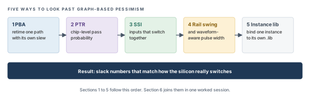
The chapter moves from the most used feature, path-based analysis, to more specialized checks. Figure 1 shows the order. Come back to it whenever you lose your place.
Key commands
Table 1 lists the commands and settings covered in this chapter, grouped by section. Do not try to memorize them now. Each one is explained when it is first needed.
| Section | Command or setting | What it does |
|---|---|---|
| 1 PBA | report_timing -retime path_slew_propagation |
Retime the reported paths with their own slews |
| 1 PBA | report_constraint -retime |
Constraint report with retimed paths |
| 1 PBA | -retime_mode exhaustive |
Search for the true worst retimed path per endpoint |
| 1 PBA | timing_pba_exhaustive_path_nworst_limit |
Paths searched per endpoint in exhaustive mode |
| 1 PBA | timing_disable_retime_clock_path_slew_propagation |
Retime data only, or data and clock |
| 1 PBA | -retime aocv, -retime aocv_path_slew_propagation |
Retime AOCV depth, or depth and slew |
| 2 PTR | set_analysis_mode -timing_robustness true |
Turn on robustness analysis |
| 2 PTR | set_delay_cal_mode -socv_lvf_mode, -socv_accuracy_mode |
Use moment LVF data and set statistical accuracy |
| 2 PTR | report_timing_robustness, report_property |
Compute the chip pass probability and read it |
| 3 SSI | set_timing_derate -input_switching |
Derate cells whose inputs switch together |
| 3 SSI | define_property, set_property |
Create and set the k_input_switching_window_* window properties |
| 4 Waveform | timing_rail_swing_checks_*_voltage_threshold |
Rail swing thresholds as ratios of VDD |
| 4 Waveform | report_constraint -check_type rail_swing |
Report signals that do not reach the rails |
| 4 Waveform | set_min_pulse_width -waveform_aware_type, reset_min_pulse_width |
Set a pulse width requirement on the real waveform, or remove it |
| 4 Waveform | report_min_pulse_width -waveform_aware_type |
Report regular, waveform-aware or both pulse width checks |
| 5 Instance library | set_instance_library, report_instance_library |
Bind instances to a library and confirm it |
1 Path-based analysis (PBA)
1.1 The concept
Every timing report starts from a simple picture. Signals travel from a launch flop, through gates and wires, to a capture flop. Each gate adds a delay. That delay depends on two things. One is the load the gate drives. The other is the slew of its input – how fast the input edge rises or falls.
A slow input edge gives a larger delay, because the gate starts switching later and switches more slowly. A fast input edge gives a smaller delay. Thus, the input slew of every gate matters for the slack of every path through it.
In graph-based analysis (GBA), the tool walks the design once, pin by pin. Each pin keeps one worst arrival and one worst slew. When two paths meet at a gate, the gate output is computed from the worst of its inputs. Every path through that gate then inherits the worst value – even a path that never had it.
Let us consider Figure 2. Two paths meet at the NAND gate U3. The input from U1 has a slow slew of 120 ps. The input from U2 has a fast slew of 30 ps. We want to time the path from FF2 to FF3, drawn in red.
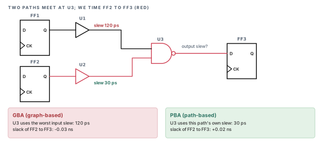
In GBA, U3 uses the worst input slew, 120 ps, to compute its delay and its output slew. Thus, the path from FF2 is charged for a slew it never sees. The slower output slew of U3 then also slows FF3's setup check. The error grows with every merge point along the path.
Path-based analysis (PBA) fixes this. It takes one path at a time and recomputes every delay along it with that path's own slews. This is called retiming a path. In Figure 2, PBA computes U3 with the 30 ps slew. The slack moves from −0.03 ns to +0.02 ns.
Think of GBA as a city map that marks every junction with its worst traffic of the day. Any route through that junction is planned with the worst jam. PBA plans each route with the traffic it would really meet.
- In a city, traffic changes over time. In STA, the slews are fixed numbers for a given corner.
- PBA is not "optimistic". It is still a worst-case analysis, only for the path's own conditions.
- PBA does not change the design. It only changes how precisely the tool computes the same path.
1.2 Why it matters
PBA removes pessimism without changing the design. A path that passes in PBA is not a real violation, so it does not need a fix. On a large design, PBA often clears many small GBA violations. Each cleared path saves an ECO change, which saves area, power and a re-run.
In most settings, the GBA slack is a safe bound on the PBA slack. In other words, PBA slack is typically equal to or better than GBA slack. Thus, GBA stays the safe first pass for the whole design. PBA is the sharper answer for the paths that matter.
However, PBA is slow. Each retimed path needs its own delay calculation for every stage. Retiming every path in a design is not practical. The tool therefore retimes a chosen set of critical paths, as we will see below.
1.3 Running PBA
PBA is requested through report_timing with the -retime option. The following command retimes the worst setup paths and writes a short summary file.
tempus> report_timing -retime path_slew_propagation \
          -max_paths 500 -nworst 5 \
          -path_type summary_slack_only -late \
          -analysis_summary_file pba.summ   ;# PBA on setup paths, summary to file
Each argument has a clear job:
-retime path_slew_propagation– retime each path, propagating its own slew from stage to stage. Without-retime, the report is plain GBA. This is the value you will use most often.-max_paths 500– the number of GBA paths the report considers. In the regular-mode description below, this plays the role of N. A larger value catches more paths but costs more run time.-nworst 5– at most this many paths per endpoint. This plays the role of M. Without it, one bad endpoint could fill the whole report with its own paths.-path_type summary_slack_only– one line per path, with slack only. This keeps a 500-path report short enough to scan.-late– setup analysis. Use-earlyfor hold. Forgetting this switch gives you the wrong check type.-analysis_summary_file pba.summ– writes a summary of the PBA run to a file. Keep it with the run, so later runs can be compared.
The mapping of N and M to -max_paths and -nworst follows the usual meaning of these options. Confirm the exact behavior with help report_timing in your installation.
The constraint report also accepts retiming. Use report_constraint -retime with a retime value, so the violation summary reflects PBA slack. Confirm the allowed values with help report_constraint.
1.4 Reading a PBA report
A retimed report can show three extra columns. Add them with the report_timing_format global or with the -format option of report_timing:
retime_slew– the slew recomputed along this path. Compare it with the GBA slew to see where the pessimism was.retime_delay– the stage delay recomputed with that slew.retime_incr_delay– the incremental delay after retiming, stage by stage.
The report header names the retime method, for example Retime Analysis {Path-Slew ...}. The line Slack Time(original) shows the GBA slack of the same path. Thus, one report shows both numbers side by side.
Retime Analysis {Path-Slew}
Slack Time(original) -0.030
Slack Time 0.020Figure 3 breaks the same path into stages. It shows where the gain comes from.
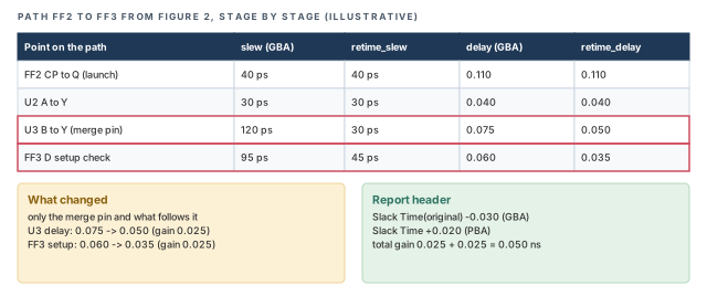
Slack Time(original) and Slack Time. Numbers are illustrative.In this illustrative case, the path gained 0.050 ns from retiming. If the gain is very large on one stage, look at that stage's retime_slew. A large drop in slew usually points to a merge pin with a slow side input.
Slack Time(original).1.5 Retiming the clock path too
PBA can retime only the data path, or the clock paths as well. Clock trees also have merge points, for example clock muxes and clock gating cells. The launch and capture clock paths can carry GBA pessimism of their own.
The variable timing_disable_retime_clock_path_slew_propagation controls this. When it is true, only the data path is retimed. When it is false, the clock paths are retimed as well.
Let us consider Figure 4. Two clocks meet at a clock mux. In this illustrative case, GBA gives the mux output the worse of the two slews, 110 ps. The launch and capture clocks of CLKA then carry a slew they never see.
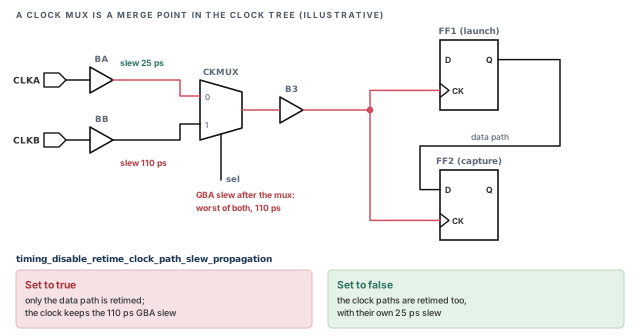
false, the launch and capture clocks are retimed with CLKA's own 25 ps slew.What to notice: The merge-point pessimism of Figure 2 also lives in the clock tree. Slews are illustrative.tempus> set timing_disable_retime_clock_path_slew_propagation false ;# retime clock tooNote the double negative in the name: "disable" set to false means clock retiming is on. It is better to retime the clock path when the clock tree has merge points with mixed slews. Otherwise, the launch and capture clocks keep their GBA pessimism, and PBA removes only part of it. Retiming the clock typically costs extra run time, so check the run time on a small path set first.
1.6 Regular and exhaustive modes
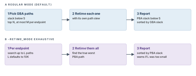
The tool has two ways to choose the paths it retimes. In regular mode, it works in three steps:
- It takes the top N GBA paths with slack below a limit S, with at most M paths per endpoint.
- It retimes each of them with its own slews.
- It reports the retimed paths whose PBA slack is still below S, sorted by GBA slack.
Figure 5 compares regular mode with the exhaustive mode described below.
The sort order matters. Let us consider four paths, shown in Table 2. Assume the slack limit S is +0.020 ns, so all four are reported. Path P1 is worst in GBA, but it gains the most from retiming. Path P3 gains very little.
| Path | GBA slack (ns) | PBA slack (ns) | Position in regular report |
|---|---|---|---|
| P1 | −0.050 | +0.010 | 1st |
| P2 | −0.040 | −0.005 | 2nd |
| P3 | −0.030 | −0.025 | 3rd |
| P4 | −0.020 | +0.004 | 4th |
The first line of the report is P1, which passes after retiming. The worst real slack, −0.025 ns, sits on the third line. Thus, do not read the top line of a regular PBA report as the worst real slack.
There is a second, quieter risk. Regular mode only retimes the paths it picked from GBA. At a busy endpoint, the worst PBA path may not be among the top M GBA paths. Regular mode can then miss it entirely.
Figure 6 shows how this happens at one endpoint.
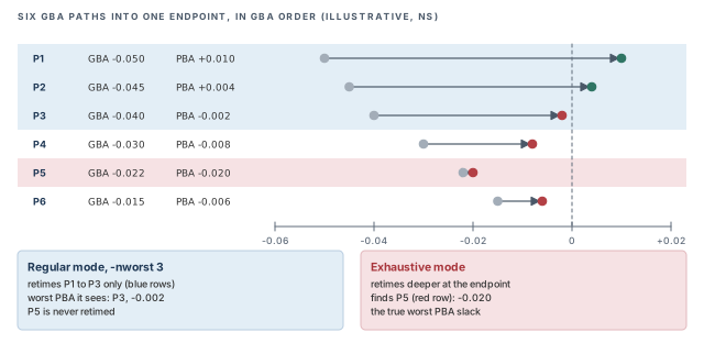
-nworst 3, regular mode retimes only P1 to P3; the worst PBA path, P5, is never retimed.What to notice: P5 gains almost nothing from retiming, so it ends up worse than every retimed path. Numbers are illustrative.In exhaustive mode, set with -retime_mode exhaustive, the tool searches for the true worst PBA path at each endpoint. It retimes up to L paths per endpoint, going deeper than the GBA order. The limit L is set with a global:
tempus> set_global timing_pba_exhaustive_path_nworst_limit 20000   ;# default is 10K
tempus> report_timing -retime path_slew_propagation -retime_mode exhaustive \
          -max_paths 100 -late   ;# true worst PBA path, sorted by PBA slack
The default limit is 10K paths per endpoint. If the L-th path at an endpoint still violates in GBA, the search may have stopped too soon. The tool then issues a warning that the result is incomplete. The exhaustive report is sorted by PBA slack, so its first line is the worst real slack.
When should you raise L? Raise it when the incomplete-search warning appears. A higher limit gives a complete answer at the cost of run time. If the warning keeps appearing, the endpoint has a huge number of near-critical paths, which is itself worth a closer look.
A beginner runs regular PBA, sees the first path pass, and assumes all paths pass. However, regular mode sorts by GBA slack. A worse PBA path can sit lower in the list, or be missed. Use exhaustive mode when you need the true worst PBA slack.
1.7 PBA with AOCV and signal integrity
PBA also changes two other parts of the calculation.
AOCV depth. With AOCV, the stage count of a path decides its derate (see Analysis Modes, CPPR and AOCV). GBA works with a pin-based count, which can differ from the real depth of one path. Thus, the AOCV derate can differ between GBA and PBA. Two retime values handle this:
-retime aocv– retime the AOCV depth of the path.-retime aocv_path_slew_propagation– retime both the AOCV depth and the slew.
The timing_aocv_analysis_mode global still controls how launch and capture depth are counted. When AOCV is on, it is better to use aocv_path_slew_propagation, because it removes both kinds of GBA pessimism together.
Signal integrity. Crosstalk depends on timing windows – the time ranges in which nets can switch (see Signal Integrity Delay Analysis). PBA recomputes the victim timing window for the path being retimed. The aggressor timing windows always stay as GBA computed them. Thus, PBA sharpens the victim side only.
Figure 7 shows why this can remove an attacker from a path.
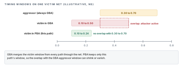
The report header then lists the active methods, for example { Path-Slew SI WP EWM }. Here, SI most likely marks crosstalk-aware retiming, and EWM the equivalent waveform model from Base Delay Calculation. Confirm every tag with help report_timing.
2 Parametric timing robustness (PTR)
2.1 The concept
A normal report gives one slack per path, computed at a fixed number of sigmas. Each path is judged on its own. However, the chip passes only if every endpoint passes at the same time, on the same piece of silicon.
Parametric timing robustness (PTR) answers that chip-level question: what is the probability that all endpoints meet timing together? A result of 0.977 means that, under the statistical model, about 977 chips in 1,000 meet timing on all endpoints.
PTR needs the tpsng license. The tool estimates the probability by Monte Carlo (MC) sampling per timing arc. In simple terms, it draws random delay values for the arcs from their statistical data. It then times the design with those values, and repeats. Figure 8 shows the loop.
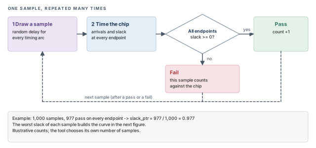
slack_ptr.What to notice: One failing endpoint makes the whole sample fail. That is why PTR is a chip-level number.Each sample gives one worst chip slack. Many samples build a curve of worst chip slack. Let us consider Figure 9. The shaded tail to the left of zero is the chance that at least one endpoint fails.
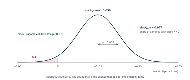
The numbers in Figure 9 can be checked by hand. Zero slack sits (0.050 − 0) / 0.025 = 2 sigma below the mean. For a normal curve, about 97.7% of samples lie above that point.
2.2 Why it matters
Fixed-sigma signoff treats each path on its own. In a large chip, many paths are each "probably fine". However, the chance that all of them pass together can be lower than the chance for any single path.
For example, assume 100 independent paths, each passing with probability 0.999. The chance that all pass is 0.999¹⁰⁰, about 0.905. Real paths share cells and are not independent, so the real number differs. Still, the example shows why a chip-level view adds information.
PTR shows that combined risk as one number. Thus, it helps the designer decide whether small residual violations really threaten yield. It also gives a common language for the discussion between designers and managers.
2.3 The library data PTR needs
PTR needs Liberty Variation Format (LVF) data – statistical delay tables inside the library. Each table gives a sigma for each combination of input slew and output load, much like a normal delay table.
A form of LVF with moments is strongly recommended. Plain sigma tables describe only the spread of a delay. Moments also describe how the mean shifts and how lopsided the distribution is. Real delay distributions are often lopsided, with a longer tail on the slow side. Moments let the samples follow that shape.
Figure 10 shows a lopsided delay and the moment that describes each of its features.
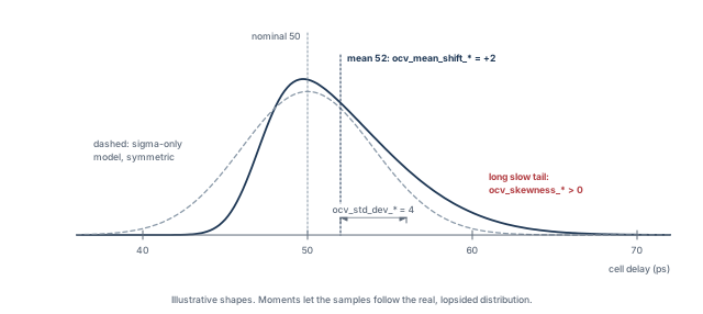
The sigma table groups are listed in Table 3.
| Group | What it describes |
|---|---|
ocv_sigma_cell_rise, ocv_sigma_cell_fall |
Sigma of the cell delay |
ocv_sigma_rise_transition, ocv_sigma_fall_transition |
Sigma of the output transition |
ocv_sigma_rise_constraint, ocv_sigma_fall_constraint |
Sigma of timing checks such as setup and hold |
ocv_sigma_retaining_rise, ocv_sigma_retaining_fall |
Sigma of the retaining delay |
ocv_sigma_retain_rise_slew, ocv_sigma_retain_fall_slew |
Sigma of the retaining slew |
These groups carry a sigma_type of early or late. An early table describes the fast side of the distribution; a late table describes the slow side. The constraint tables are the exception: they have no early or late split.
The moment groups are:
ocv_std_dev_*– the standard deviation of the value.ocv_mean_shift_*– how far the mean moves from the nominal value.ocv_skewness_*– how lopsided the distribution is.
The moment groups have no sigma_type. They can sit in the same library as the ocv_sigma_* groups, so one library can serve both normal SOCV runs and PTR.
2.4 Running PTR
The following script turns PTR on and runs it on one path group.
tempus> set_analysis_mode -timing_robustness true   ;# enable robustness analysis
tempus> set timing_disable_retime_clock_path_slew_propagation false   ;# PBA on clock too
tempus> set_delay_cal_mode -socv_lvf_mode moments   ;# use moment LVF data
tempus> set_delay_cal_mode -socv_accuracy_mode ultra   ;# statistical accuracy setting
tempus> set P1 [report_timing_robustness -check_type setup -path_group R2R \
          -target_PTR 0.95 -run_time_limit 15]   ;# setup PTR for group R2R
tempus> report_property $P1   ;# print the result properties
The setup lines each have a reason:
set_analysis_mode -timing_robustness true– turns the robustness engine on. Without it,report_timing_robustnesshas nothing to work with.timing_disable_retime_clock_path_slew_propagation false– retimes the clock paths too, so clock pessimism does not distort the probability.-socv_lvf_mode moments– tells delay calculation to read the moment tables. Without moment data in the library, this setting has nothing to use.-socv_accuracy_mode ultra– selects the statistical accuracy level used in this flow. Confirm the other levels and their run-time cost withhelp set_delay_cal_mode.
The options of report_timing_robustness are:
-check_type setup– the kind of check to evaluate. Use the check type that worries you, typically setup at the slow corner.-path_group R2R– the path group to analyze; here, register-to-register paths. One group at a time keeps the run small.-target_PTR 0.95– the pass probability you aim for. The quantile in the result is reported at this target.-run_time_limit 15– a limit on the run time of the analysis. Confirm its unit withhelp report_timing_robustness.
The result is stored in the variable P1. It holds five properties, read with report_property:
slack_mean– the mean of the worst-slack distribution.slack_stddev– its standard deviation, the width of the curve.slack_skewness– how lopsided it is. A negative skew means a longer tail toward failing slack.slack_ptr– the pass probability, the share of samples where every endpoint passes.slack_quantile– the slack at the target probability. In Figure 9, 95% of samples have slack above 0.009 ns.
Let us check the quantile by hand. For a normal curve, the 5% point lies 1.645 sigma below the mean. Thus, 0.050 − 1.645 × 0.025 ≈ 0.009 ns. A positive quantile at the target means the target is met.
It is better to start PTR on one path group, with a run-time limit. Sampling is expensive. A small first run shows whether the library data and settings are correct before you scale up.
A beginner loads a library with only ocv_sigma_* tables and sets -socv_lvf_mode moments. The moment data the setting expects is missing. Check the library for ocv_std_dev_*, ocv_mean_shift_* and ocv_skewness_* groups first.
3 Simultaneous switching inputs (SSI)
3.1 The concept
A library delay table is measured with one input switching while the other inputs stay still. This is a clean, repeatable setup for characterization. In real circuits, however, two inputs of a gate can switch at almost the same moment. The output then moves at a different speed from the table.
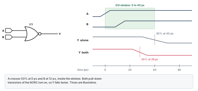
Let us consider the NOR2 gate in Figure 11. Its output Y falls when an input rises. A NOR2 has two pull-down transistors in parallel, one per input. If A rises alone, one transistor discharges Y. If A and B rise together, two transistors discharge Y in parallel, so Y falls faster.
In Figure 11, the single-input delay is 40 ps. With both inputs switching, it is 28 ps. Thus, the real delay is 30% smaller than the library table says. The exact speed-up depends on the cell and on how close the two edges are.
3.2 Why it matters
A faster output edge shortens the data path. For a setup check, a shorter path is good news. For a hold check, a shorter data path is the dangerous case. Data may change before the capture flop has held it.
Thus, ignoring simultaneous switching can hide real hold violations. Those failures do not depend on clock frequency, so the chip would fail at any speed. SSI modeling applies a derate to chosen cells when their inputs switch together.
3.3 Command breakdown
The derate uses set_timing_derate with the -input_switching option:
tempus> set_timing_derate 0.5 -fall -data -early -delay_corner tt_800 \
          -power_domain pdDefault \
          -input_switching [get_lib_cells NOR2*]   ;# halve early fall delay on NOR2
Each part of the command narrows where the derate applies:
0.5– the derate factor applied to the delay. A factor below 1 makes the delay smaller, which is the pessimistic direction for hold.-fall– apply only to falling output transitions. For a NOR2, the falling output is the case with parallel pull-downs.-data– apply only on data paths, not clock paths.-early– apply in early analysis, which is used for hold checks.-delay_corner tt_800– apply only in this delay corner. Other corners keep their own settings.-power_domain pdDefault– apply only to cells in this power domain.-input_switching [get_lib_cells NOR2*]– the library cells that get the SSI treatment. Here, every NOR2 variant.
The value 0.5 is an example. The right factor for your library should come from characterization or from your library team. Too small a factor creates false hold violations; too large a factor misses real ones.
3.4 The switching window
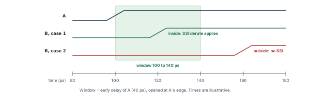
Two inputs count as simultaneous when the second one switches inside a switching window. The window opens at the edge of the first input. By default, the window equals the early delay of the pin that switches first.
For example, assume A switches at 100 ps, and the early delay from A is 40 ps. The window then runs from 100 ps to 140 ps. If B switches at 120 ps, it falls inside the window. If B switches at 160 ps, it does not, and no SSI derate applies.
Figure 12 draws both cases.
To size the window per library, define and set a float property:
tempus> define_property -type float -object_type lib k_input_switching_window_rise   ;# rise
tempus> define_property -type float -object_type lib k_input_switching_window_fall   ;# fall
tempus> set_property [get_libs slow] k_input_switching_window_rise 1.1   ;# window factor
define_property -type float -object_type lib– creates the property on library objects. It must exist before it can be set.k_input_switching_window_riseandk_input_switching_window_fall– one property for rising and one for falling inputs.set_property [get_libs slow] ... 1.1– sets the value for the libraryslow. Confirm withhelphow the value 1.1 scales the default window in your installation.
These property settings persist when the constraints are written out as SDC. Thus, a later session that reads that SDC keeps the same windows.
3.5 When the window is tested
The clocks of the two inputs decide whether the tool tests the window at all. Figure 13 lists the five cases.
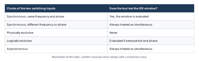
The reasoning follows from what the tool can know:
- Synchronous, same frequency and phase – the arrival times are known, so the tool tests the window.
- Synchronous, different frequency or phase – the edges have no single fixed offset to test, so the tool treats them as always simultaneous.
- Physically exclusive – the clocks never exist on the chip together, so the inputs never switch together.
- Logically exclusive – the tool tests the window if the period and phase match.
- Asynchronous – nothing rules out an overlap, so the tool assumes one.
3.6 Combining derates and the GBA–PBA link
An SSI derate multiplies with any user derate on the same arc. For example, a user derate of 0.90 and an SSI derate of 0.50 give 0.90 × 0.50 = 0.45. A 40 ps arc then becomes 40 × 0.45 = 18 ps in early analysis. The report shows the product in the "User Derate" column.
Figure 14 shows this rule together with the GBA–PBA rule below.
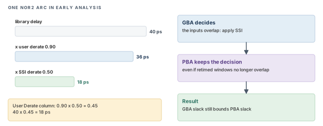
The decision to apply SSI is taken in GBA. If GBA applies it to an arc, PBA applies it too, even if the retimed windows would no longer overlap. This keeps the rule that GBA bounds PBA. Thus, a PBA report may still show an SSI derate that looks surprising at first.
A beginner sets the SSI derate without checking the clock relationships. With asynchronous clocks, every candidate arc counts as simultaneous. The derate then applies far more widely than expected. Review the clock groups before trusting the hold results.
4 Rail swing and waveform-aware pulse width
Both checks in this section look at the real voltage shape of a waveform, not only at its 50% crossing. The usual delay numbers say when a signal crosses the middle. These checks ask how far and how long it really goes.
4.1 Rail swing checks
A healthy signal swings almost fully between ground and the supply. Let us consider Figure 15. A weak driver feeds a long wire and many receivers. It needs a long time to charge all that capacitance.
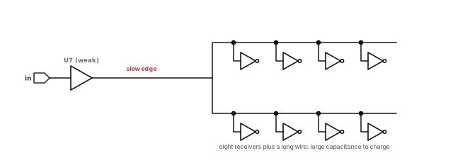
If the input of the driver toggles again before the output settles, the output never reaches the rail. A receiver then sees a level that is neither a clean 1 nor a clean 0. It may switch late, draw extra current, or fail to switch at all. The rail swing check catches this.
Figure 16 shows two signals. The green signal reaches both rails. The red signal peaks at 0.88 of the supply and then settles at 0.20, so it misses both thresholds.
The thresholds are globals, written as ratios of VDD:
tempus> set timing_rail_swing_checks_high_voltage_threshold 0.95   ;# ratio of VDD
tempus> set timing_rail_swing_checks_low_voltage_threshold 0.05    ;# ratio of VDD
tempus> report_constraint -check_type rail_swing -all_violators    ;# list failures
timing_rail_swing_checks_high_voltage_threshold 0.95– a rising signal must reach 95% of VDD. With VDD = 0.80 V, that is 0.76 V.timing_rail_swing_checks_low_voltage_threshold 0.05– a falling signal must drop below 5% of VDD, 0.04 V in the same example.report_constraint -check_type rail_swing -all_violators– lists every signal that misses a threshold.
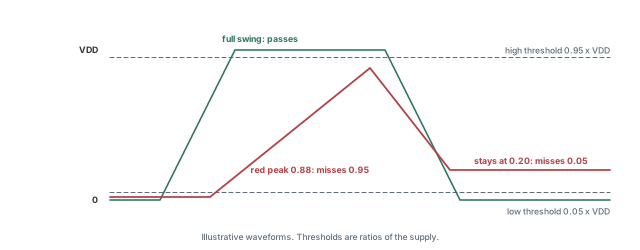
Because the thresholds are ratios, the same setting works at every voltage corner. The usual fixes are a stronger driver, a smaller load, or buffering the long net.
4.2 Waveform-aware minimum pulse width
A minimum pulse width (MPW) check makes sure a clock pulse stays high, or low, long enough for a flop to respond. The regular check measures the width at the 50% crossings. However, a slow edge spends part of that time far from the rail. There, the flop may not yet see a valid level.
Let us consider Figure 17. At 50%, the pulse is 0.32 ns wide. At the 75% level, it is only 0.28 ns wide. Assume a 0.30 ns requirement. The regular check passes with 0.02 ns margin. The waveform-aware check fails by 0.02 ns.
The width loss comes from both edges. In Figure 17, each edge takes 0.08 ns to go from 0 to 100%. Moving the measurement from 50% to 75% costs a quarter of each edge. That is 0.02 ns on the rise and 0.02 ns on the fall.
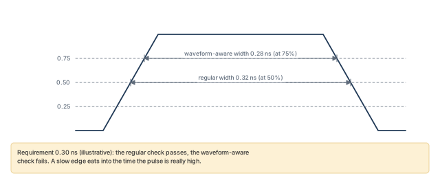
The measurement levels are globals. The requirement and the report take a -waveform_aware_type option:
tempus> set timing_waveform_aware_pulse_width_checks_high_voltage_level 0.75   ;# high level
tempus> set timing_waveform_aware_pulse_width_checks_low_voltage_level 0.25    ;# low level
tempus> set_min_pulse_width 0.1 [get_clocks clk1] \
          -waveform_aware_type absolute   ;# requirement on clk1
tempus> report_min_pulse_width -waveform_aware_type both \
          -pins FF1/CP -verbose   ;# regular and waveform-aware
The script uses a 0.1 ns requirement on clk1 as a syntax example. Each setting does one job:
timing_waveform_aware_pulse_width_checks_high_voltage_level 0.75– a high pulse is measured where the signal is above 75% of VDD.timing_waveform_aware_pulse_width_checks_low_voltage_level 0.25– a low pulse is measured where the signal is below 25% of VDD.set_min_pulse_width ... -waveform_aware_type– takesabsoluteorsource_width_ratio. An absolute requirement is a fixed time. A ratio requirement is relative to the source pulse width. Confirm the exact meaning withhelp set_min_pulse_width.reset_min_pulse_width– removes such requirements, for example before reading a corrected constraint set.report_min_pulse_width -waveform_aware_type– takesregular,waveform_awareorboth. The default isregular, so a waveform-aware check is not reported unless you ask for it.-pins FF1/CP -verbose– limits the report to one clock pin and prints the detail of the measurement.
A beginner sets the waveform-aware levels and runs report_min_pulse_width with no option. The report shows only the regular check, because regular is the default. Ask for waveform_aware or both explicitly.
5 Binding instances to a library
5.1 The concept
Normally, every instance of a cell takes its timing from the library set of its delay corner. If the netlist uses AND2X1, every AND2X1 instance uses the same table. This is simple and usually correct.
Sometimes one instance needs a different library. It may run at another voltage, or it may be a macro characterized at a slightly different corner. The command set_instance_library binds chosen instances to a named library, while the rest of the design keeps the normal one.
5.2 Why it matters
Three situations call for it:
- Multi-supply designs without power intent – some instances run at another voltage, but no power-intent file tells the tool. Without a binding, those instances are timed at the wrong voltage.
- Macros without a matching PVT – a macro library exists only at a corner that does not match the rest. The binding lets the corner still use it.
- Patching mis-bound instances – an instance picked up the wrong library and needs a quick correction, without rebuilding the library sets.
In each case, the wrong library gives wrong delays. That can hide real violations or create false ones on the affected paths.
5.3 How it works
Figure 18 shows the flow. The binding lives in a small Tcl file. That file is passed to the delay corner, so the binding applies per corner.
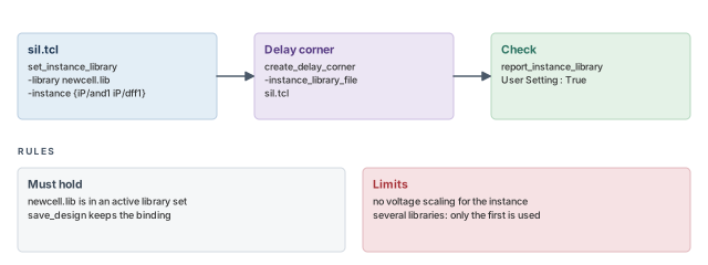
report_instance_library, which shows "User Setting : True" when applied.What to notice: The library must already be in an active library set.set_instance_library -library newcell.lib -instance {iP/and1 iP/dff1} ;# bind two instances-library newcell.lib– the library the instances should use.-instance {iP/and1 iP/dff1}– the hierarchical names of the instances to bind.
tempus> create_delay_corner -name slow_max -library_set complete_library_set \
          -pg_net_voltages {VDD2@0.9 VDD1@0.9} \
          -instance_library_file sil.tcl   ;# corner with instance bindings
tempus> report_instance_library -inst {iP/and1 iP/dff1} ;# check the binding-library_set complete_library_set– the normal library set for this corner.-pg_net_voltages {VDD2@0.9 VDD1@0.9}– names a voltage for each supply net in this corner, here 0.9 V for both.-instance_library_file sil.tcl– reads the binding file for this corner.report_instance_library -inst– prints the binding for the named instances. The lineUser Setting : Truemeans the binding was applied.
Keep four rules in mind:
- The library, here
newcell.lib, must be part of an activecreate_library_set. Otherwise the binding cannot take effect. save_designwrites the binding under${::IMEX::silLibVar}/mmmc/, so a restored session keeps it.- There is no voltage scaling for a bound instance. The library must already be at the right voltage.
- If several libraries are given, only the first is used. List one library per binding.
Always run report_instance_library right after loading the corner. A binding that silently failed leaves the instance on its old library, and nothing else in the timing report will tell you.
set_instance_library in a side file, pass it with -instance_library_file, and confirm with report_instance_library. The library must be in an active library set.6 Worked example: are these failures real?
Let us join the features in one session. The assumptions are written as comments at the point of use.
The task. A block has 12 setup violations of up to −25 ps after GBA. It also has a clock pulse-width concern on FF1, and NOR2 cells on a hold-critical bus. The design is loaded with SOCV and moment LVF libraries (see SOCV and Wire Variation).
Step 1 – retime the setup failures
We start with regular PBA, because it is fast and shows how much pessimism GBA added. We retime the clock path too, so both sides of each check are sharp.
tempus> set timing_disable_retime_clock_path_slew_propagation false   ;# retime clock too
tempus> report_timing -retime path_slew_propagation -max_paths 200 -nworst 3 \
          -path_type summary_slack_only -late \
          -analysis_summary_file setup_pba.summ   ;# retime the top setup paths
What to look for. Compare Slack Time(original) with the new slack for each path. Assume nine paths now pass. The report is sorted by GBA slack, so the order may hide the worst PBA path.
Step 2 – confirm the true worst path
Regular mode may have missed a path, and its order is not the PBA order. Exhaustive mode answers both concerns.
tempus> set_global timing_pba_exhaustive_path_nworst_limit 10000   ;# keep the default 10K
tempus> report_timing -retime path_slew_propagation -retime_mode exhaustive \
          -max_paths 20 -late   ;# sorted by PBA slack
What to look for. First, check the log for the incomplete-search warning. If none appears, the first path is the true worst PBA path. Assume exhaustive mode confirms three failing paths. Only those three need an ECO.
Step 3 – model simultaneous switching on the bus
The hold-critical bus uses NOR2 cells whose inputs come from the same clock. SSI can make them faster than the tables say.
# Assuming the bus is clocked by one synchronous clock, so the window is evaluated
tempus> set_timing_derate 0.5 -fall -data -early -delay_corner tt_800 \
          -power_domain pdDefault \
          -input_switching [get_lib_cells NOR2*]   ;# faster fall when inputs switch together
tempus> report_timing -early -max_paths 20   ;# hold paths with SSI applied
What to look for. Check the "User Derate" column on the NOR2 arcs. A value of 0.5 shows that SSI applied. Any new hold failure here is a real risk, not pessimism.
Step 4 – check the clock pulse on its real waveform
tempus> set timing_waveform_aware_pulse_width_checks_high_voltage_level 0.75   ;# high level
tempus> set timing_waveform_aware_pulse_width_checks_low_voltage_level 0.25    ;# low level
tempus> report_min_pulse_width -waveform_aware_type both \
          -pins FF1/CP -verbose   ;# both checks on FF1
What to look for. If the regular check passes but the waveform-aware check fails, the clock edge at FF1 is too slow. The fix is usually on the clock driver, not on the data path.
Step 5 – measure the remaining risk
tempus> set_analysis_mode -timing_robustness true   ;# enable PTR
tempus> set_delay_cal_mode -socv_lvf_mode moments   ;# moment LVF
tempus> set P1 [report_timing_robustness -check_type setup -path_group R2R \
          -target_PTR 0.95 -run_time_limit 15]   ;# probability for R2R
tempus> report_property $P1   ;# slack_ptr, slack_quantile and the rest
What to look for. Read slack_ptr and slack_quantile. If slack_ptr is above the 0.95 target, the team has a measured basis to discuss the three small violations. Otherwise, the ECO goes ahead. Either way, the decision now rests on numbers, not on guesswork.
7 Common mistakes and how to catch them
Table 4 gathers the mistakes from this chapter. Each row gives the symptom you would see first.
| Symptom | Likely cause | Fix |
|---|---|---|
| First PBA path passes, but a later one fails | Regular mode is sorted by GBA slack | Use -retime_mode exhaustive for the true worst |
| Exhaustive run warns the result is incomplete | The L-th path at an endpoint still fails in GBA | Raise the exhaustive path limit global (Section 1.6) |
| PBA removes less pessimism than expected | Only data is retimed | Set the clock-retime variable (Section 1.5) to false |
| PBA and GBA disagree on AOCV derates | Depth not retimed | Use an aocv retime value (Section 1.7) |
| PTR fails to run or looks unrealistic | No LVF, or no moment data | Load LVF with moments; set the moments LVF mode |
| SSI derate applies almost everywhere | Asynchronous clocks always count as simultaneous | Review the clock groups |
| SSI seen in PBA but not expected | SSI was applied in GBA, so PBA keeps it | This is intended; it keeps GBA bounding PBA |
| No waveform-aware results in the report | Default -waveform_aware_type is regular |
Request waveform_aware or both |
| Signal misses a rail on a long net | Weak driver on a heavy load | Upsize the driver, reduce the load or buffer the net |
report_instance_library shows no user setting |
Library not in an active library set | Add it to create_library_set |
| Bound instance ignores its voltage | No voltage scaling for bound instances | Provide a library at the right voltage |
| Second library in a binding is ignored | Only the first library is used | Bind one library per instance list |
8 Interview preparation
Each pin keeps only the worst slew and arrival, so every path through a merge pin inherits the worst value.
- A path with a fast slew is timed as if it had the slow slew of another branch.
- A slower input slew gives a larger delay, so the path looks worse than it is.
- The error adds up at every merge point along the path.
-retime path_slew_propagation do?It retimes each reported path, propagating that path's own slew through every stage.
- The report keeps the GBA slack as
Slack Time(original). - The columns
retime_slew,retime_delayandretime_incr_delayshow the recomputed values.
Not necessarily. Regular mode sorts the retimed paths by GBA slack.
- A path that is worst in GBA may gain the most from retiming and pass.
- Regular mode can also miss a path that was not among the top GBA paths.
- Exhaustive mode sorts by PBA slack and finds the true worst path.
timing_pba_exhaustive_path_nworst_limit control?How many paths per endpoint exhaustive PBA may search; the default is 10K.
- If the last searched path still fails in GBA, the tool warns that the result is incomplete.
- Raising the limit gives a complete answer at the cost of run time.
It recomputes the victim window for the path being retimed, but aggressor windows stay as GBA computed them.
- Thus, PBA sharpens only the victim side of crosstalk.
- The header lists the methods used, for example
{ Path-Slew SI WP EWM }.
The probability that all endpoints meet timing together, estimated by sampling arc delays; it needs LVF, ideally with moments.
- One failing endpoint makes a sample fail, so the result is a chip-level number.
- It reports
slack_mean,slack_stddev,slack_skewness,slack_ptrandslack_quantile. - It needs the
tpsnglicense.
The constraint tables, and the moment tables such as ocv_std_dev_*, which carry no sigma_type at all.
- The other sigma groups carry
sigma_typeearly or late. - Moment tables can sit in the same library as the
ocv_sigma_*groups.
When both inputs rise together, two pull-down transistors discharge the output, so it falls faster.
- A faster data edge shortens the data path.
- A shorter data path can create hold violations, which is why the derate is early.
For synchronous clocks with the same frequency and phase, and for logically exclusive clocks with the same period and phase.
- Asynchronous clocks, or synchronous clocks with different frequency or phase, always count as simultaneous.
- Physically exclusive clocks never do.
0.45, because the two derates multiply.
- A 40 ps arc becomes 40 × 0.45 = 18 ps.
- The product appears in the "User Derate" column.
It measures the pulse at a level such as 75% of the supply, where slow edges make the pulse narrower.
- Each slow edge loses part of its time between the 50% and 75% levels.
- The report shows it only with
-waveform_aware_type waveform_awareorboth.
set_instance_library, and what are its limits?For multi-supply designs without power intent, macros with no matching PVT, or patching mis-bound instances.
- The library must be in an active library set.
- There is no voltage scaling, and only the first of several libraries is used.
- Confirm the binding with
report_instance_libraryand the lineUser Setting : True.
Chapter recap
Key takeaways
- GBA keeps the worst slew at each pin. PBA retimes a path with its own slews and removes that pessimism.
- Regular PBA is sorted by GBA slack. Exhaustive PBA finds the true worst path and is sorted by PBA slack.
- Retime the clock path too, and retime AOCV depth when AOCV is on.
- PTR turns many per-path slacks into one chip-level pass probability, using LVF data.
- SSI derates gates whose inputs switch together. Clock relationships decide when the window is tested.
- Rail swing and waveform-aware pulse width look at the real voltage shape of a signal.
set_instance_librarybinds chosen instances to a library, with no voltage scaling.
Command recap
| Command or setting | Purpose |
|---|---|
report_timing -retime path_slew_propagation |
Retime paths with their own slews |
-retime aocv, -retime aocv_path_slew_propagation |
Retime AOCV depth, or depth and slew |
-retime_mode exhaustive |
True worst PBA path per endpoint |
report_constraint -retime |
Retimed constraint report |
timing_pba_exhaustive_path_nworst_limit |
Exhaustive search limit per endpoint (default 10K) |
timing_disable_retime_clock_path_slew_propagation |
Retime data only, or data and clock |
set_analysis_mode -timing_robustness true |
Enable PTR |
set_delay_cal_mode -socv_lvf_mode, -socv_accuracy_mode |
Moment LVF and accuracy for PTR |
report_timing_robustness, report_property |
Run PTR and read its result |
set_timing_derate -input_switching |
SSI derate on chosen library cells |
define_property, set_property with k_input_switching_window_* |
Size the SSI window per library |
timing_rail_swing_checks_*_voltage_threshold |
Rail swing thresholds |
report_constraint -check_type rail_swing |
Report rail swing failures |
timing_waveform_aware_pulse_width_checks_*_voltage_level |
Waveform-aware measurement levels |
set_min_pulse_width, reset_min_pulse_width |
Set or remove pulse width requirements |
report_min_pulse_width -waveform_aware_type |
Report regular, waveform-aware or both |
set_instance_library, report_instance_library |
Bind instances to a library and check it |
Compact glossary
| Term | Meaning |
|---|---|
| Slew | How fast an edge rises or falls |
| GBA | Graph-based analysis: one worst value per pin, shared by all paths |
| PBA | Path-based analysis: each path retimed with its own values |
| Retiming | Recomputing a path's delays with its own slews |
| Exhaustive PBA | Searching each endpoint for the true worst retimed path |
| PTR | Parametric timing robustness: probability that all endpoints pass |
| Monte Carlo | Estimating a probability by repeating random samples |
| LVF | Liberty Variation Format: statistical delay data in the library |
| Moments | Mean shift, standard deviation and skewness of a delay |
| Quantile | The slack value that a given share of samples stays above |
| SSI | Simultaneous switching inputs: inputs that change at almost the same time |
| Switching window | Time range after the first input edge in which a second edge counts as simultaneous |
| Rail swing | How close a signal gets to the supply and ground levels |
| MPW | Minimum pulse width: the shortest allowed high or low pulse |
Practical perspective
On a real project, PBA is the first step after GBA closure, not the last. Teams usually run regular PBA often and exhaustive PBA before each signoff milestone. SSI, rail swing and waveform-aware pulse width checks are added when the library and the technology call for them. PTR adds a different way to discuss residual risk. It turns "a few picoseconds of violation" into a probability that managers can weigh against an ECO.
What comes next
So far, every check has assumed a stable supply and fresh transistors. The next chapter, Power Domains, IR Drop and Aging, removes those assumptions. We look at paths that cross voltage domains, at supply droop, and at transistors that slow down with age.