Chapter overview
So far, every cell in our examples ran at one fixed supply voltage. Real chips are not that simple. A modern block often has several power domains, each with its own supply. The supply also sags while the chip switches, and transistors slow down as they age.
Each of these effects changes cell delay. Let us consider one path that passes with 0.08 ns of slack at nominal voltage. Bind it to the wrong library, ignore a 5% droop or forget ten years of wear. In each case, that slack can turn negative. Thus, signoff must time each cell at the voltage it really sees.
This chapter covers four jobs. First, we set up multi-supply timing with CPF or a power-aware netlist, and we check which CPF features the tool reads. Then we time inter-power-domain (IPD) paths, add IR drop with Tempus PI, and finish with aging-aware STA.
The common thread is simple. Every section answers one question: at what voltage, and with which library, is this cell timed? If you keep that question in mind, the many commands in this chapter fall into place.
Learning objectives
- Explain why supply voltage, IR drop and aging all change cell delay.
- Load a multi-supply design with CPF or a power-aware (PGV) netlist, and validate the library binding.
- List the CPF versions and the CPF features the tool does not support for timing.
- Define an IPD path and set up the two-run IPD flow with voltage sweeps and exclusions.
- Use
check_ipd_logicto find paths that would explode the number of voltage combinations. - Run the four Tempus PI steps, from an IR budget to IR-aware ECO.
- Set the IR-drop data types, windows, scalers and thresholds, and predict which setting wins.
- Build an aging stress profile, set activity, and choose the aging analysis options.
- Generate a SPICE deck to correlate aging results.
Chapter roadmap
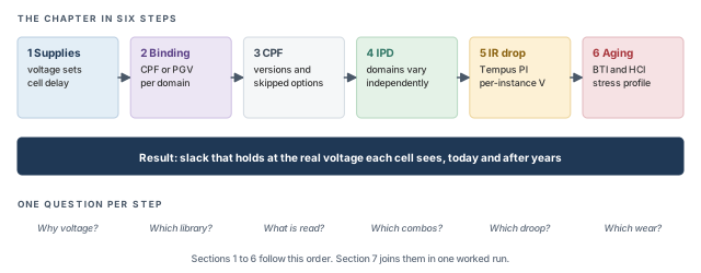
The chapter moves in six steps, from why voltage matters to aging. Figure 1 shows the order. Come back to it whenever you lose your place.
Key commands
Table 1 lists the main commands by section. Each one is explained where it is first used.
| Section | Command | What it does |
|---|---|---|
| 2 Multi-supply | read_power_intent -cpf, read_mmmc -cpf, read_power_domain -cpf |
Read CPF power intent |
| 2 Multi-supply | set_lib_binding_by_voltage, infer_pgv_power_intent |
Bind libraries from a power-aware netlist |
| 2 Multi-supply | report_instance_library, report_delay_calculation -voltage |
Check which library and voltage each instance uses |
| 2 Multi-supply | set_op_cond, set_timing_library |
Bind libraries per domain without MMMC |
| 3 CPF support | define_library_set -user_attributes, getCPFUserAttributes |
Attach and read CPF user attributes |
| 4 IPD | set_analysis_mode -enable_ipd, set_ipd_rail_voltage |
Turn on IPD and define voltage sweeps |
| 4 IPD | create_pg_net_group, report_ipd_configuration |
Group rails and review the setup |
| 4 IPD | create_ipd_configuration, write_ipd_scope, read_ipd_scope |
Build, save and load the IPD scope |
| 4 IPD | check_ipd_logic, report_timing -ipd |
Audit risky crossings and report IPD paths |
| 5 Tempus PI | update_delay_corner -irdrop_data, set_delay_cal_mode |
Load IR-drop data and choose how it is used |
| 5 Tempus PI | set_power_analysis_mode, set_rail_analysis_mode, analyze_rail |
Run power and rail analysis |
| 5 Tempus PI | set_irdrop_mode |
Guard-band and filter IR-drop values |
| 6 Aging | set_analysis_mode -aging true |
Turn on aging-aware timing |
| 6 Aging | create_aging_stress_profile, set_aging_activity |
Describe stress over the product's life |
| 6 Aging | set_aging_analysis_mode, create_spice_deck |
Control aging analysis and SPICE correlation |
1 How supply voltage shapes timing
1.1 The concept
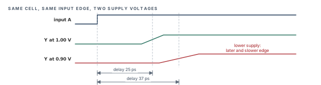
A cell switches by charging and discharging the capacitance on its output. The transistors supply that charge as current. The supply voltage sets how hard they can drive. Thus, a lower supply means less current, a slower edge and a longer delay.
Let us consider Figure 2. The same cell sees the same input edge at two supplies. At 1.00 V the delay is 25 ps. At 0.90 V the delay grows to 37 ps, and the output edge is slower too. A 10% drop in supply gave about a 50% rise in delay here.
A simple picture helps. Think of filling a bucket from a tap. Lower water pressure fills the same bucket more slowly. The bucket is the load capacitance, and the pressure is the supply voltage.
The slower output edge matters as much as the delay. That edge becomes the input slew of the next cell. Thus, a low supply on one cell also slows the cells it drives.
1.2 Four ways the voltage can differ
The supply a cell sees can differ from "nominal" in four ways:
- Power domains – a power domain (PD) is a group of cells on one supply. Different domains can run at different voltages on purpose. For example, a CPU core may run at 0.8 V while an always-on block runs at 1.0 V.
- Domain voltage ranges – each domain's voltage can move within its own range, independently of other domains. A domain may be set to 0.7 V in a low-power mode and 0.8 V in a fast mode.
- IR drop – current through the resistance of the power grid lowers the local supply. This sag is called IR drop, after Ohm's law (V = I × R).
- Aging – transistors slowly degrade under voltage and temperature stress. The same cell becomes slower over the years, even at the same supply.
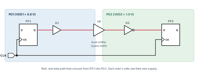
Figure 3 shows a path that crosses from one domain to another. A level shifter (LS) translates the signal between the two voltage levels. It sits on the boundary, so it connects to both supplies.
1.3 Why it matters
Each of the four effects moves delay in a known direction. A lower supply makes a cell slower, which hurts setup. A higher supply makes a cell faster, which can hurt hold. Thus, the voltage must be right for both early and late timing.
The danger is that none of these mistakes produces an error. A wrong voltage simply gives a wrong delay. The report looks normal, and the problem shows up only in silicon.
2 Multi-supply timing setup
2.1 Why binding matters
The tool picks a library for each instance. This choice is called binding. In a single-supply design, binding is trivial: every cell uses the library for that one supply. In a multi-supply voltage (MSV) design, binding comes from the power intent – a description of the domains, their supplies and their voltages.
Let us consider cell U2 in Figure 3. It sits in PD2 at 1.0 V. If the tool binds it to the 0.8 V library, every U2 delay comes from the wrong table. The slack is wrong, but the run completes cleanly.
The tool accepts power intent in two common forms:
- CPF – a separate power-intent file that names domains, nets and operating conditions.
- PGV – a power-aware Verilog netlist (
power_aware.v) whose cells carry their power and ground connections. The tool infers the power intent from it.
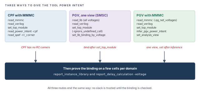
Figure 4 shows the three routes this section covers. They differ in how the intent arrives, but they all end with the same check.
2.2 The CPF flow
Let us walk through a CPF-based MMMC session. One point needs care first. CPF describes domains and voltages, but it has no RC corners. Thus, you create RC corners with create_rc_corner and read parasitics per corner with read_spef -rc_corner.
tempus> set_multi_cpu_usage -local_cpu 8      ;# 8 local CPUs (also spelled -localCpu)
tempus> read_mmmc abc.tcl                      ;# views, corners, RC corners
tempus> read_verilog abc.v                     ;# netlist
tempus> set_top_module abc                     ;# link the design
tempus> read_power_intent -cpf xyz.cpf         ;# domains, supplies, voltages
tempus> read_spef -rc_corner rc_wc design.spef ;# parasitics for one RC corner
tempus> update_timing -full                    ;# full timing update
tempus> report_analysis_views                  ;# confirm the active views
tempus> report_instance_library U2             ;# which library U2 is bound to
tempus> report_delay_calculation -voltage -from U2/A -to U2/Y  ;# voltage used
tempus> report_timing                          ;# only now trust the slack
tempus> save_design -overwrite abc_lp          ;# save the session
The order has a reason at each step:
- The MMMC file comes first, because views and RC corners must exist before anything refers to them.
- The netlist and
set_top_modulebuild the linked design that the power intent will describe. read_power_intent -cpfthen maps each instance to its domain and its supply.- Parasitics are read per RC corner, because CPF does not create those corners.
- The three reports after
update_timingconfirm the views, the library and the voltage, in that order.
Do not trust multi-supply slack before you check the binding. Run report_instance_library and report_delay_calculation -voltage on a few cells in each domain. A wrong binding gives clean-looking but wrong numbers.
There is a second way to import CPF. It reads the CPF together with the MMMC setup:
tempus> read_mmmc -cpf xyz.cpf     ;# MMMC objects plus power intent
tempus> read_verilog abc.v         ;# netlist
tempus> set_top_module abc         ;# link
tempus> init_design                ;# build the design database
The second route reads the power intent together with the view setup, which some teams find easier to maintain. Validate the binding the same way after either route.
Noise libraries in cdB format attach either through the library set or through CPF user attributes. The CPF support section shows the attribute form.
2.3 Binding without MMMC
Without MMMC, you bind libraries per domain with set_op_cond and set_timing_library:
tempus> set_op_cond cond1 -library lib1 -powerdomain pd1   ;# one condition for pd1
tempus> set_timing_library -max Max -min Min               ;# max and min libraries
tempus> set_op_cond -max c1 -maxlibrary L1 -min c2 -minLibrary L2 \
-powerdomain pd1 ;# max and min for pd1- The first line names an operating condition (
cond1), the library that defines it (-library lib1) and the domain it applies to (-powerdomain pd1). set_timing_library -max Max -min Minnames the libraries used for late (max) and early (min) timing.- The last line sets separate max and min conditions and libraries for one domain in a single command. Note the mixed case of
-maxlibraryand-minLibrary; type them exactly as shown.
This form is typically found in older scripts. For new work, MMMC keeps corners, libraries and domains together, which is easier to review.
2.4 The PGV flow for one view (SMSC)
SMSC means single mode, single corner – one view. In the PGV flow, the netlist already shows which supply net each cell uses. You read every library at every voltage, and the tool binds by voltage.
tempus> read_lib {lib_0p8.lib lib_0p9.lib}       ;# all libraries, all voltages
tempus> read_verilog power_aware.v               ;# netlist with power pins
tempus> set_top_module -ignore_undefined_cell top ;# link, skip undefined cells
tempus> read_sdc func.sdc                        ;# constraints
tempus> read_spef design.spef                    ;# parasitics
tempus> set_lib_binding_by_voltage -power_net_voltages {VDD1@0.8 VDD2@0.9} \
          -process 1 -temperature 125            ;# bind each net to a voltage
tempus> report_timing ;# slack with voltage bindingread_libloads all voltage versions of the libraries. The tool needs every candidate before it can choose.-ignore_undefined_celllets the link step continue past cells it cannot define, as its name suggests. Confirm the exact behavior withhelp set_top_module.-power_net_voltages {VDD1@0.8 VDD2@0.9}gives each power net its voltage, in the formnet@volts.-process 1 -temperature 125set the process and temperature used to pick the library.set_lib_binding_by_voltagemust come afterset_top_module. Before linking, the tool has no power nets to bind.
Behind the scenes, the tool infers an internal CPF 1.0e description. It makes one domain per power net, named pd_<net>, and one library set per domain. For VDD1, the domain is pd_VDD1.
For different early and late voltages, use -early_power_net_voltages and -late_power_net_voltages. The tool then builds separate early and late library sets and operating conditions.
2.5 The PGV flow with MMMC
With MMMC, the voltages go into the delay corner through -pg_net_voltages:
create_delay_corner -name dc1 -library_set libset_all -opcond slow \
-opcond_library std_v2.lib -pg_net_voltages {VDD1@0.535 VDD2@0.7} -rc_corner rctempus> read_mmmc view_definition_template.tcl ;# corner with PG net voltages
tempus> read_verilog power_aware.v ;# netlist with power pins
tempus> set_top_module -ignore_undefined_cell top ;# link
tempus> infer_pgv_power_intent ;# build power intent from the netlist
tempus> set_analysis_view -setup {av1} -hold {av1} ;# must come after inference
tempus> report_timing ;# timing with inferred intent- Only one active view is allowed in this flow. For several views, run several sessions.
- Process and temperature come from the corner's
-opcond, not from separate options. - For early and late voltages, use
-early_pg_net_voltagesand-late_pg_net_voltages. set_analysis_viewmust followinfer_pgv_power_intent. The reason is simple: the views need the inferred domains to exist.
- You may see the inference step described as
add_pg_netlist_power_intent. The command to type isinfer_pgv_power_intent. - Some copied templates show
constraint_modewithout its leading dash. Always write it as-constraint_mode.
2.6 Proving the binding
Whichever route you take, finish with the same check. It is quick, and it prevents the most expensive kind of error.
- Pick two or three cells in each domain, including one cell on each side of a level shifter.
- Run
report_instance_libraryon each. The library name should match the domain's voltage. - Run
report_delay_calculation -voltageon one arc of each. The voltage used should match the domain. - If any cell is wrong, fix the power intent and rerun before reading slack.
report_instance_library and report_delay_calculation -voltage before trusting any slack.3 CPF support in the tool
3.1 Why CPF support needs checking
A CPF file serves many tools. Implementation tools insert isolation cells, power switches and retention flops. Power tools estimate leakage and IR limits. A timing tool needs only part of that information.
Thus, the tool reads CPF for timing and skips some options. A skipped option is not an error. However, if you expect it to change the timing, you will be misled. This section lists what the tool reads and what it skips.
3.2 Versions and their key options
CPF has grown over several versions. Table 2 shows the update_power_domain options that mark each version. If your CPF uses one of these options, it needs at least that version.
| CPF version | Key update_power_domain options |
|---|---|
| 1.0 | -internal_power_net |
| 1.0e | -primary_power_net, -secondary_domains |
| 1.1 | -base_domains, -equivalent_power_nets, -stage_1_on_resistance, -stage_2_on_resistance |
3.3 What is not supported
The tool skips the options in Table 3. A dash means nothing is listed as unsupported for that version. Where an entry names one version, such as (1.0e), it applies to that version only.
| CPF command | Unsupported in CPF 1.0 | Unsupported in CPF 1.0e / 1.1 |
|---|---|---|
create_bias_net |
-driver, IR limits |
– |
create_ground_nets, create_power_nets |
-voltage (ground), -internal (ground), IR limits |
– |
create_isolation_rule |
-isolation_target |
-no_condition (1.0e) |
create_nominal_condition |
-pmos_bias_voltage, -nmos_bias_voltage |
-state, bias |
create_operating_corner |
– | -ground_voltage, bias |
create_power_domain |
-power_up_states |
-power_up_states, -active_state_condition |
define_isolation_cell |
-non_dedicated |
-no_enable (1.0e) |
define_level_shifter_cell |
-always_on_pin, -output_voltage_input_pin |
ground ranges, -input_ground_pin, -output_ground_pin, -power (1.0e) |
define_power_switch_cell |
– | -enable_pin_bias, -gate_bias_pin |
define_state_retention_cell |
-always_on_pin, -clock_pin, -restore_check, -save_check |
-always_on_components |
identify_power_logic |
– | entry reads "only -type isolation" |
set_power_target |
not applicable | -leakage, -dynamic |
set_switching_activity |
-clock_pins, -toggle_percentage, -mode |
-clock_pins, -toggle_percentage |
update_isolation_rules |
-combine_level_shifting |
– |
update_power_domain |
power-up times, bias nets, -rail_mapping |
bias nets, -transition_* options |
update_power_mode |
activity files, power and IR limits | activity files, power limits |
update_power_switch_rule |
– | -gate_bias_net |
update_state_retention_rules |
– | -set_rest_control |
set_power_mode_control_group |
-groups |
-groups |
In CPF 1.0e and 1.1, four whole commands are also unsupported: set_equivalent_control_pins, set_floating_ports, set_input_voltage_tolerance and define_power_clamp_cell.
The identify_power_logic entry is brief. Confirm with help identify_power_logic whether -type isolation is the only accepted form or the skipped one.
Notice the pattern in Table 3. Most skipped items are about bias voltages, power-up states, IR limits and switching activity. Many of these serve power and implementation tools. However, some, such as bias voltages, can change delay in silicon. If your design relies on one of them, confirm how the timing setup accounts for it.
3.4 Attaching noise and AOCV data through CPF
define_library_set -user_attributes can attach cdB noise data and AOCV data to a CPF library set. This keeps all library data for a domain in one place. To read user attributes back, use getCPFUserAttributes or ::CPF::getCpfUserAttr.
Before signoff, scan the CPF for the options in Table 3. It is better to know a setting is ignored than to assume it changed the timing.
4 Inter-power-domain (IPD) analysis
4.1 The concept
In the earlier sections, each domain had one fixed voltage per corner. In a real chip, each domain's supply moves within its own range. The domains also move independently – one can be high while another is low.
Let us consider two domains. PD1 can be 0.7 V or 0.8 V. PD2 can be 0.9 V or 1.0 V. A path that crosses from PD1 to PD2 sees four possible combinations. Each combination is called a voltage signature. Figure 5 shows them.
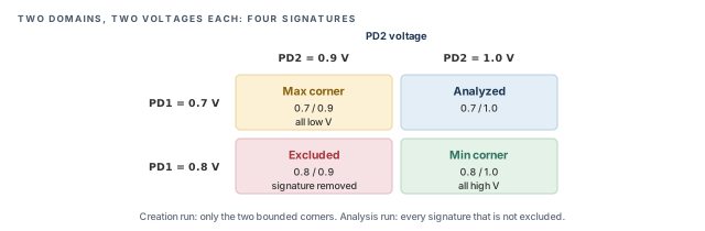
The number of signatures grows fast. Two domains with two voltages each give 2 × 2 = 4. Three domains with three voltages each give 3 × 3 × 3 = 27. This growth is the main cost of IPD, and much of the flow exists to control it.
4.2 Why it matters
A path inside one domain is worst at that domain's low voltage. However, a crossing path can be worst at a mixed signature.
Let us consider a setup check with illustrative numbers. The data launches in PD1 and the capture flop sits in PD2. At PD1 = 0.7 V the data arrives late. At PD2 = 1.0 V the capture clock arrives early, which leaves less time.
- The all-low corner slows the capture clock too, so some of the late data is forgiven.
- The mixed signature (0.7 V / 1.0 V) slows only the data. It can fail where both bounded corners pass.
Figure 6 puts numbers on this. The clock period is 1.80 ns and the setup time is 0.05 ns. The required time is 1.80 + capture clock latency − 0.05.
- At PD1 = 0.7 V, the launch clock takes 0.40 ns and the data takes 1.65 ns. The data arrives at 2.05 ns.
- At PD2 = 0.9 V, the capture clock takes 0.40 ns, so the required time is 2.15 ns. The slack is +0.10 ns.
- At PD2 = 1.0 V, the capture clock takes only 0.25 ns, so the required time is 2.00 ns. The slack is −0.05 ns.
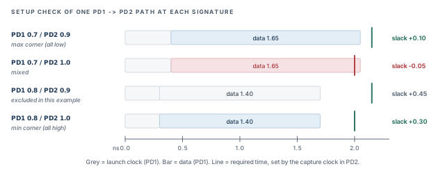
Thus, crossing paths need every signature, not just the two bounded corners.
4.3 What counts as an IPD path
An IPD path is one that the tool must time over the signatures:
- A data path that crosses more than one domain.
- A clock path that crosses more than one domain, when one of these holds:
- there is no CPPR common point, or
- the CPPR point has a different transition, or
- a domain transition happens after the CPPR common point.
The CPPR common point is the last shared point of the launch and capture clocks, from Analysis Modes, CPPR and AOCV. When both clocks share their domains up to that point, the shared part cancels out. Only the parts after it can see different voltages.
Figure 7 compares the two cases for a clock. In panel A, the clock enters PD2 before it splits, so both branches see the same supply. In panel B, the clock splits in PD1 and only one branch enters PD2. That branch can be fast or slow on its own, so the tool must time it over the signatures.
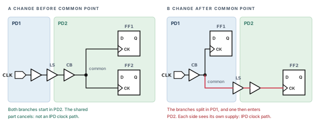
Watch paths that pass through two or more domains after the clock common point. One stray path of this kind can explode the number of corners the tool must time. Find such paths early with check_ipd_logic.
4.4 How it works: two runs
Timing the whole design at every signature would be very slow. Most paths do not cross domains at all. Thus, the flow uses two runs, shown in Figure 8.
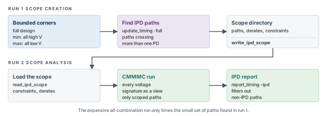
- Run 1, scope creation – the full design is timed at two bounded corners. The min corner has every domain at its high voltage. The max corner has every domain at its low voltage. The tool finds the IPD paths and writes the scope.
- Run 2, scope analysis – a CMMMC run over all signatures, timing only the scoped paths.
The saving is large. Run 1 costs two corners on the full design. Run 2 costs every signature, but only on the small scoped set.
4.5 Command breakdown: defining the sweep
These commands set up IPD. Turn IPD on at the top of the script.
tempus> set_analysis_mode -enable_ipd true            ;# first line of the script
tempus> set_ipd_rail_voltage -sweep { PD1 {0.7 0.8} PD2 {0.9 1.0} }   ;# ranges
tempus> set_ipd_rail_voltage \
          -exclude_voltage_signatures { {PD1 0.8 PD2 0.9} }   ;# never-used combination
tempus> create_pg_net_group -name PG1 -pg_nets {pgn1 pgn2}   ;# treat as one rail
tempus> report_ipd_configuration                      ;# review the setup
set_analysis_mode -enable_ipd trueturns the IPD machinery on. Put it at the top, so every later setting is read in IPD mode.-sweeplists the voltages to try for each rail. Each extra voltage multiplies the signature count, so list only real operating points.-exclude_voltage_signaturesremoves combinations that never happen in the product. For example, the power manager may never run PD1 high while PD2 is low. Excluding such a signature saves runtime without losing coverage.create_pg_net_groupgroups nets into one rail. Crossings inside a group are ignored. Use it for nets that always carry the same voltage, so they do not count as separate domains.report_ipd_configurationprints the setup. Read it before the long run, because a typo in a rail name wastes the whole run.- With CPF or 1801 (UPF) power intent, the rail names are the domains' primary power nets.
4.6 Command breakdown: run 1, scope creation
tempus> read_library my_libs.lib            ;# libraries (help read_library for form)
tempus> read_verilog top.v                  ;# netlist
tempus> set_top_module top                  ;# link
tempus> update_library_set -timing {lib_0p7.lib lib_0p8.lib} -append  ;# all voltages
tempus> read_power_intent -cpf top.cpf   ;# or read_power_domain / infer_pgv_power_intent
tempus> set_analysis_mode -enable_ipd true  ;# IPD on
tempus> create_pg_net_group -name PG1 -pg_nets {pgn1 pgn2}            ;# rail groups
tempus> set_ipd_rail_voltage -sweep { PD1 {0.7 0.8} PD2 {0.9 1.0} } \
          -exclude_voltage_signatures { {PD1 0.8 PD2 0.9} }           ;# signatures
tempus> create_ipd_configuration -bounded_corners   ;# min and max bounded corners
tempus> set_interactive_constraints_modes \
          [all_constraints_modes -active]     ;# next SDC applies to all modes
tempus> source bounding_corner_constraints.sdc      ;# constraints for the corners
tempus> set_timing_derate -cell_delay 0.9 \
          -delay_corner [all_delay_corners -active]   ;# derate on every active corner
tempus> read_spef top.spef                  ;# parasitics
tempus> update_timing -full                 ;# find the IPD paths
tempus> write_ipd_scope -include_derates -include_constraints -bounded_corners \
          -overwrite ipd_scope              ;# save paths, derates, constraints
The script follows a clear logic:
- Read the design, then append every voltage's library with
update_library_set -timing ... -append. Each signature needs its own library. - Load the power intent, so the tool knows which cell belongs to which domain.
- Define rails and signatures, then let
create_ipd_configuration -bounded_cornersbuild the two bounded corners. - Apply constraints and derates to all active modes and corners, then time the design.
write_ipd_scopesaves the found paths.-include_deratesand-include_constraintssave those settings too, so run 2 does not need them again.-overwritereplaces an older scope folder.
This script spells two commands as read_library and set_interactive_constraints_modes [all_constraints_modes -active]. Other chapters use read_lib and set_interactive_constraint_modes. Confirm the spelling in your installation with help.
4.7 Command breakdown: run 2, scope analysis
tempus> set_analysis_mode -enable_ipd true      ;# IPD on
tempus> read_ipd_scope ipd_scope                ;# load the scope from run 1
tempus> create_ipd_configuration -load_constraints -load_derates  ;# reuse them
tempus> update_timing -full                     ;# time scoped paths at all signatures
tempus> report_timing -ipd ;# report IPD paths onlyread_ipd_scopeloads the folder written in run 1.create_ipd_configuration -load_constraints -load_deratesrebuilds every signature view with the saved constraints and derates. Thus, run 1 and run 2 time the same paths under the same rules.- Use
report_timing -ipdand not plainreport_timing. The reason is that graph-based analysis may still time some non-IPD paths. The-ipdswitch filters them out.
4.8 Auditing crossings with check_ipd_logic
check_ipd_logic finds the crossing patterns that make IPD expensive or risky. Run it after update_timing with power intent loaded.
tempus> check_ipd_logic -multi_pd_type all \
-outfile ipd_logic_check_report -verbose ;# audit risky crossings-multi_pd_type allchecks every kind of multi-domain pattern.-outfilenames the report file.-verboseadds detail to the report.
It flags three patterns:
- Multiple data or clock domain crossings on one path.
- Similar crossings on divergent clock paths.
- More than two domains after the clock common point.
It also writes ipd_logic_check.tcl, which holds report_timing commands for the flagged paths. Source that file to look at each flagged path in detail.
Run check_ipd_logic before the first full IPD run. One unexpected clock crossing can multiply the run time. It is far cheaper to fix that crossing early than to wait for a run that takes far too long.
check_ipd_logic.5 IR-drop-aware timing with Tempus PI
5.1 The concept
The power grid is a mesh of metal wires, and metal has resistance. When many cells switch at once, current flows through that resistance and the local supply sags. By Ohm's law, the drop is current times resistance.
Let us consider one hot spot. A cluster draws 50 mA through a grid path of 1 Ω. The drop is 50 mA × 1 Ω = 50 mV. On a 1.0 V supply, that is a 5% loss right where those cells switch.
The drop is not the same everywhere. Cells near a power pad or in a quiet area see almost the full supply. Cells in a busy area far from a pad see the deepest sag.
5.2 Why it matters
The traditional approach adds one flat margin for IR drop to every cell. That margin is either too large or too small. Too large, and you waste power and area fixing paths that are fine. Too small, and a cell in a hot spot fails in silicon. Thus, real per-instance voltages give honest slack where it matters.
Figure 9 shows the supply at one instance over three busy moments.
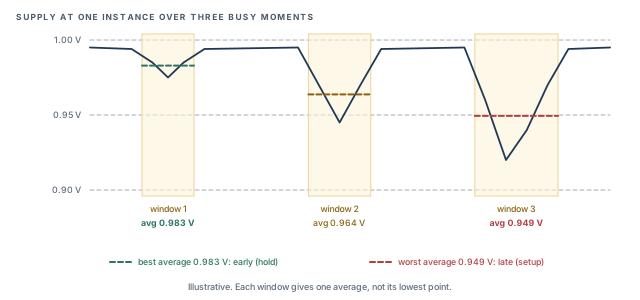
Tempus PI (TPI) turns this droop into a voltage per instance, called the effective instance voltage (EIV). STA then times each cell at its own EIV. The EIV is an average over a window. A cell's delay depends on the supply during its transition, not at one instant.
In Figure 9 the instance sees three windows, with averages of 0.983 V, 0.964 V and 0.949 V. The highest average is the best average, and the lowest is the worst average. Thus, early timing uses 0.983 V and late timing uses 0.949 V. How the windows are drawn depends on the window setting, covered in Step 2.
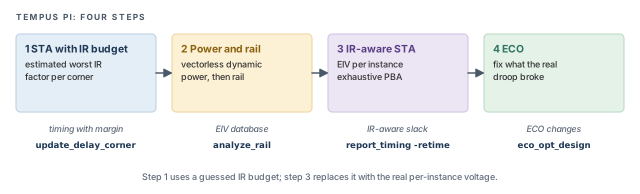
5.3 How it works: four steps
Figure 10 shows the flow. Step 1 uses a guessed IR budget. Steps 2 and 3 replace the guess with real voltages. Step 4 fixes what the real voltages break.
What Tempus PI needs
- Licenses – Tempus XL, Voltus XL and Tempus PI. Setting
set_power_analysis_mode -enable_tempus_pi truechecks out the others. - Libraries – characterized at three or more voltages below nominal, in steps of about 10% to 15%. These points let the tool cover the expected sag.
- Power method – it works only with
-method dynamic_vectorless.
Step 1 – STA with an IR budget
After the usual import (LEF, view definition, Verilog, DEF, SPEF), add an estimated worst IR-drop factor to the delay corner:
tempus> update_delay_corner -name DC_wc_1p00 \
          -early_estimated_worst_irDrop_factor 0.15 \
          -late_estimated_worst_irDrop_factor 0.15   ;# 15% budget, early and late
tempus> update_timing -full                          ;# timing with the budget
This gives a first, pessimistic view. It shows which paths are sensitive to IR drop before any power data exists. The factor defaults to 0, so without this step no IR budget is applied.
Step 2 – power and rail analysis
This step runs vectorless dynamic power, then a rail analysis that writes the EIV database. Vectorless means the tool estimates switching from default activity rates, without a simulation file.
tempus> set_power_output_dir dynVecLessPowerResults           ;# power results folder
tempus> set_power_analysis_mode -method dynamic_vectorless -disable_static true \
          -enable_state_propagation true -enable_tempus_pi true \
          -power_grid_library {techonly.cl stdcells.cl macros.cl}  ;# grid models
tempus> set_default_switching_activity -input_activity 0 \
          -clock_gates_output 2.0 -seq_activity 0.2          ;# default activity
tempus> set_dynamic_power_simulation -resolution 50ps -period 320ns  ;# simulated span
tempus> report_power                                         ;# run power analysis
The comments give the purpose each option name suggests. Confirm units and allowed values with help for each command.
-method dynamic_vectorlessis the only method Tempus PI accepts.-disable_static trueskips static power, so the run focuses on dynamic switching current.-power_grid_librarylists the grid models for the technology, standard cells and macros.set_default_switching_activitysets how often inputs, clock-gate outputs and sequential cells switch.set_dynamic_power_simulationsets the time step (-resolution) and the span simulated (-period).
tempus> set_rail_analysis_mode -method dynamic -accuracy hd \
          -analysis_view AV_wc_1p00 -power_grid_library {techonly.cl stdcells.cl macros.cl} \
          -enable_rlrp_analysis true -temperature 125 \
          -eiv_eval_window switching -eiv_method {bestavg worstavg}   ;# EIV settings
tempus> set_pg_nets -net VDD_AO -voltage 1 -threshold 0.95 -force    ;# when no CPF
tempus> set_pg_nets -net VSS -voltage 0.0 -threshold 0.05 -force     ;# ground net
tempus> set_rail_analysis_domain -name ALL -pwrnets {VDD_AO} -gndnets VSS  ;# one domain
tempus> set_power_pads -net VDD_AO -format xy -file VDD_AO.pp        ;# pad locations
tempus> set_dynamic_rail_simulation -resolution 50ps                 ;# rail time step
tempus> set_power_data -scale 1 -format current \
          [glob dynVecLessPowerResults/*.ptiavg]                     ;# currents from power
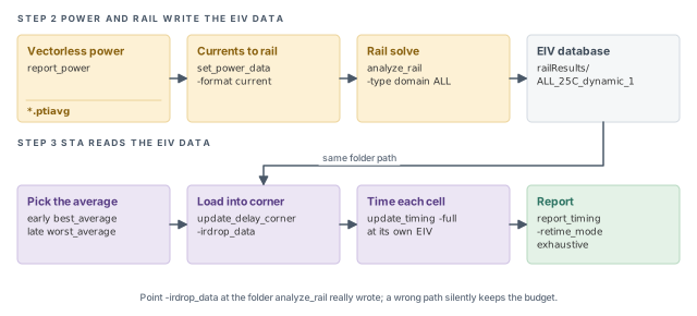
tempus> analyze_rail -output ./railResults -type domain ALL ;# write EIV data-eiv_eval_window switchingpicks the window used to average the supply. The other value iselapse. The choice changes the result, so make it on purpose.-eiv_method {bestavg worstavg}asks for both the best and the worst average, for early and late timing.set_pg_netsdefines supply and ground nets when no CPF gives them.set_power_padstells the rail solver where current enters the grid.set_power_datafeeds the current waveforms from step 2A into the rail solver.analyze_railsolves the grid and writes the EIV data into the output folder.
Figure 11 follows the data through steps 2 and 3. Power writes current files, the rail solver turns them into the EIV database, and STA reads that folder. The folder path is the only link between the two halves, so it must be exact.
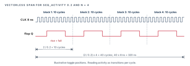
The simulated period follows a rule. The number of cycles is (2 / sequential activity) × N, where N is a multiplier you choose. The period is that cycle count times the dominant clock period.
For example, with -seq_activity 0.2 and N = 4, the tool needs (2 / 0.2) × 4 = 40 cycles. With an 8 ns dominant clock, the period is 40 × 8 = 320 ns – the value in the script. Figure 12 draws this span.
Let us read the activity as transitions per clock cycle. A flop with activity 0.2 then makes about two transitions in 10 cycles. That is one rise and one fall – a full switching pattern. N repeats the pattern, so a shorter window would miss many switching events.
Several options have a second spelling that you may meet in scripts:
-clock_gates_output_ratioand-sequential_activityfor the two activity options.analyze_rail -output_dirfor-output.set_rail_analysis_domain -domain_name,-power_netsand-ground_nets.-power_grid_librariesfor-power_grid_library.read_mmmcfollowed byinit_designfor the import.
Step 3 – IR-aware STA
Now load the EIV data into the delay corner and choose how it is used:
tempus> set_delay_cal_mode -early_irdrop_data_type best_average \
          -late_irdrop_data_type worst_average          ;# early: best, late: worst
tempus> update_delay_corner -name DC_wc_1p00 \
          -irdrop_data railResults/ALL_25C_dynamic_1    ;# real rail output folder
tempus> update_timing -full                             ;# time at each EIV
tempus> report_analysis_summary                         ;# overall summary
tempus> report_timing -max_paths 200000 -retime path_slew_propagation \
-retime_mode exhaustive -max_slack 0 ;# exhaustive PBA, failing paths- Best average for early timing and worst average for late timing gives each check its own honest worst case.
-irdrop_datapoints at the rail output folder. Always point it at the real folder thatanalyze_railwrote.update_delay_corneralso accepts-timing_condition {TC1}to target one timing condition.- The final
report_timinguses exhaustive path-based analysis on up to 200,000 failing paths. This removes graph-based pessimism before you start fixing.
Step 4 – IR-aware ECO
tempus> set_eco_opt_mode -retime path_slew_propagation -pba_effort high \
          -allow_multiple_incremental true -verbose true \
          -eco_file_prefix tempus_pi        ;# PBA-based ECO settings
tempus> checkPlace       ;# check placement legality first
tempus> deleteFiller     ;# remove filler cells to make room
tempus> eco_opt_design -setup   ;# fix setup with IR-aware timing
The ECO works on path-based timing with the real voltages. checkPlace and deleteFiller prepare the layout so new or larger cells have room. The -eco_file_prefix tempus_pi option names the output files, so they are easy to tell apart. Signoff ECO covers these ECO options in depth.
5.4 Command breakdown: IR-drop controls
Table 4 lists the set_delay_cal_mode options for IR drop. Where the table says "suggested by name", the meaning comes from the option name; confirm it with help set_delay_cal_mode.
| Option | Values and default | What it controls |
|---|---|---|
-irdrop_data_type |
best_average, worst, best, average, worst_average; default worst |
Which EIV value is used |
-early_irdrop_data_type, -late_irdrop_data_type |
same values | Separate choice for early and late |
-irDrop_window_based |
none, late, early, both |
Window-based IR values for that side (suggested by name) |
-irDrop_default_scaler |
0 to 1; default 0 (plus early_ and late_ forms) |
A default IR scaler (suggested by name) |
-irDrop_value_check_threshold |
default 0.25 | Warns with IMPDC-3280 above it; does not clamp |
-irDrop_value_guard_threshold |
default 1 | Clamps values above it |
-use_diff_volt_in_eiv_timing_analysis |
default false |
Different voltages in EIV timing (suggested by name) |
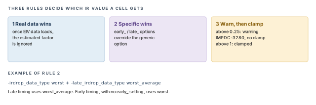
The two thresholds are a safety net. The check threshold raises a warning so you can inspect a suspicious value. The guard threshold actually limits the value. Figure 13 sums up how these rules combine.
The delay corner holds the data itself:
-irdrop_data,-early_irdrop_data,-late_irdrop_data– the EIV data folders, shared or per side.-estimated_worst_irDrop_factor– default 0, withearly_andlate_forms. It is ignored once EIV data is loaded.
set_irdrop_mode adds guard bands and filters:
tempus> set_irdrop_mode -corner DC_wc_1p00 -data \
          -irdrop_guard_band_scale_factor {VDD_AO@1.1} \
-irdrop_min_threshold {VDD_AO@0.01} ;# per-rail scale and minimum-cornernames the delay corner the setting applies to.-clockor-datalimits the setting to clock or data cells. Teams may treat clock cells more strictly, because a clock error affects many paths.-irdrop_guard_band_scale_factor {rail@f}scales the drop on a rail. A factor above 1 adds margin.-irdrop_min_threshold {rail@abs}sets an absolute threshold value per rail.- Each option also has
early_andlate_forms.
The values 1.1 and 0.01 above are illustrative.
Two precedence rules catch beginners. First, an early_ or late_ option always beats the generic option. Second, the EIV window (switching or elapse) changes the result, so choose it on purpose.
5.5 Refinements for better accuracy
User-defined critical paths (UDCP). Vectorless power guesses where switching happens. You can tell power analysis which timing paths matter, so it pays attention to them. Set it before report_power:
tempus> set_power_analysis_mode \
          -user_defined_critical_paths \
          [report_timing -collection -max_paths 100]   ;# paths for power to focus on
tempus> report_power      ;# power now focuses on those paths
The value 100 is illustrative. If you set UDCP after report_power, the power run has already finished without it.
Proximity aggressors. Cells near a victim can deepen its droop when they switch together. This flow builds an aggressor database first:
tempus> redirect -quiet {puts "setvar proximity_level 10"} > rail.inc   ;# include file
tempus> set_advanced_rail_options \
          -voltus_rail_include_file_begin ./rail.inc   ;# pass the file to the rail engine
tempus> analyze_resistance -domain ALL -output_dir agg_db -method rlrp  ;# aggressor DB
tempus> set_power_analysis_mode \
          -specify_aggressor_db_path agg_db/ALL_25C_reff_1   ;# use the aggressor DB
tempus> report_power                                                    ;# rerun power
The steps are simple. Write a small include file and pass it to the rail engine. Build the aggressor database, point power analysis at it, and rerun power.
Sequential activity from a vector run. The default sequential activity is only a guess. You can measure it from a vector-based run instead. Use a power include file:
ChipPwr rActivityCalculationCycleCountFix 1
ChipPwr rReportInstanceInGateVcdFlow 1tempus> set_power_include_file pm.inc ;# results go to voltus_power.stateprop.statsThe measured statistics land in voltus_power.stateprop.stats. A measured activity makes the cycle-count rule above more trustworthy.
-irdrop_data at the real rail output.6 Aging-aware timing
6.1 The concept
Transistors wear out slowly. Two effects matter most for timing:
- BTI (bias temperature instability) – grows while a transistor is held on, at high voltage and temperature.
- HCI (hot carrier injection) – grows each time the transistor switches.
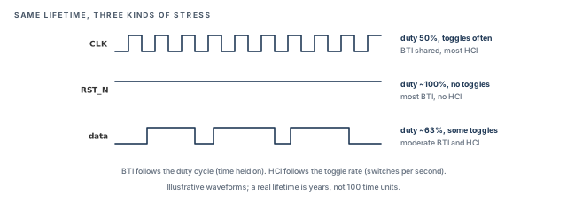
Both make cells slower over time. Thus, the analysis needs to know how each net behaves. For BTI, the key number is the duty cycle – the fraction of time a signal is high. For HCI, it is the toggle rate – switches per second.
Let us consider two nets. A clock with a 50% duty cycle stresses its pull-up and pull-down devices equally. A reset net that stays high for years stresses one side all the time. The second net ages more for BTI, even though it never toggles.
Figure 14 adds a data net between the two. The clock gives the most HCI, because it switches most often. The reset net gives the most BTI and no HCI. The data net sits in between on both counts.
6.2 Why it matters
A path that passes on day one can fail after years in the field. Products with long lifetimes – automotive, for example – often sign off at an aged condition. Aging-aware STA predicts that slack today, while fixes are still cheap.
A flat aging margin has the same problem as a flat IR margin. Nets that are rarely stressed get too much margin, and heavily stressed nets get too little. Activity-based aging puts the margin where the stress really is.
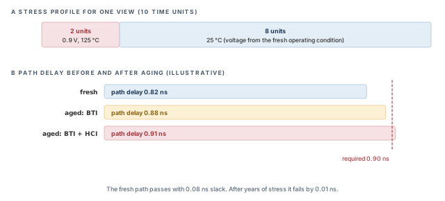
Figure 15 shows a stress profile and its effect on one path.
6.3 What aging analysis needs
- Fresh libraries in CCSN or ECSM-N format.
- Aging libraries from Liberate advanced aging characterization. The aged library name must match the fresh one.
- Power intent – PGV, UPF or CPF. The tool needs each cell's supply to judge its stress.
Attach the aging library to the fresh one as an incremental library:
tempus> create_library_set -name ls1 -timing fresh.lib \
          -liberty_incremental {{age {{age.lib ff105C}}}}   ;# MMMC form
tempus> read_lib fresh.lib -liberty_incremental {{age {age.lib}}}   ;# non-MMMC form
The fresh library gives the base delay. The incremental aging library tells the tool how that delay changes under stress. Copy the nested braces exactly; they group the library with its condition.
6.4 Command breakdown: stress profile
A stress profile describes the product's life as segments. Each segment has a duration and, optionally, a voltage and temperature.
create_aging_stress_profile [-views views] [-early] [-late]
    [-bti_pmos_scale v] [-bti_nmos_scale v]
    [-hci_pmos_scale v] [-hci_nmos_scale v]
{segment ...}tempus> create_aging_stress_profile -view view1 \
{{{duration 2} {voltage {VDD 0.9 VSS 0.0}} {temperature 125}} \
{{duration 8} {temperature 25}}} ;# 2 units hot, then 8 units cool-views(written-viewin the example) chooses the views the profile applies to.-earlyand-lateapply the profile to early or late timing only.- A segment's voltage and temperature are optional. When missing, the fresh operating condition is used. In the example, the second segment takes its voltage from the fresh condition.
- The four
-bti_*and-hci_*scales range from 0 to 1, with a default of 1. A scale below 1 reduces that effect for that device type.
The example reads naturally. The product spends 2 time units hot and stressed, at 0.9 V and 125 °C. It then spends 8 units cool, at 25 °C. Together, the two segments describe the stress over the whole life.
6.5 Command breakdown: activity
set_aging_activity [-views v] [-min_duty_cycle v] [-max_duty_cycle v]
[-min_toggle_rate v] [-max_toggle_rate v] -net nets
get_aging_activity [-views v] -net nets
report_aging_activity [-duty_cycle] [-toggle_rate] [-views v] -net nets [-out_file f]set_aging_activitygives a net a duty-cycle range and a toggle-rate range.get_aging_activityreads back what the tool will use for a net.report_aging_activityprints duty cycle, toggle rate or both, and can write them to a file with-out_file.
The defaults matter, because most nets never get a user value:
- Duty cycle at primary inputs – 50% by default, with a default range of min 0.0 and max 1.0.
- Clock duty cycle – taken from the SDC clock waveform. A user value beats the SDC.
- Toggle rate (for HCI) – default min 0.0 and max 1e8 per second. Clocks toggle twice per period.
For example, a 500 MHz clock has a 2 ns period. It toggles twice per period, so its toggle rate is 1e9 per second.
Figure 16 shows how clock duty cycle travels. It propagates along the clock until it reaches a special net or an endpoint.
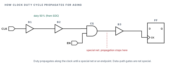
A special net is the output of a multi-input cell on the clock path, or a net you set yourself. The reason is that a clock gate's output depends on its enable. Thus, the input duty cycle no longer tells the whole story.
6.6 Command breakdown: analysis options
set_aging_analysis_mode controls how activity spreads and which effects are included. Table 5 lists the options.
| Option | Values and default | Effect |
|---|---|---|
-activity_propagation_mode |
probabilistic, worst_case |
How duty and toggle values spread through logic |
-sequential_activity_propagation |
true, false; by default activity resets at sequential outputs |
Carry activity through flops |
-min_duty_cycle, -max_duty_cycle |
value | Duty-cycle range for nets |
-sequential_min_duty_cycle, -sequential_max_duty_cycle |
value | Duty-cycle range at sequential outputs |
-min_toggle_rate, -max_toggle_rate |
value | Toggle-rate range for nets |
-sequential_min_toggle_rate, -sequential_max_toggle_rate |
value | Toggle-rate range at sequential outputs |
-recovery |
true |
Model recovery; needs OMI, URI or Liberate libraries |
-type |
bti, hci, all; default all |
Which aging effects to include |
-constraints |
true; off by default |
Age setup and hold checks; needs aged constraint arcs |
-use_fixed_duty_cycle |
true |
Use fixed duty-cycle values |
A few options deserve a closer look:
- Propagation mode.
probabilisticspreads activity through logic by probability.worst_case, as its name suggests, assumes the most stressful values. Worst case is typically safer but more pessimistic. - Sequential propagation. By default, activity resets at sequential outputs, and the sequential min and max values apply there. Turn propagation on only when you trust the activity through the flops.
- Recovery. BTI partly recovers when stress is removed.
-recovery truemodels this, but only with library types that support it. - Constraints. Setup and hold checks can age too.
-constraints trueincludes this, but only if the libraries have aged constraint arcs.
TMI libraries are not recovery-aware. With TMI, model recovery through the stress-profile scales instead of -recovery true.
6.7 The aging flow
tempus> read_view_definition view_def.tcl    ;# views and corners
tempus> read_verilog test.v                  ;# netlist
tempus> set_top_module test                  ;# link
tempus> infer_pgv_power_intent               ;# PGV power intent
tempus> set_analysis_view -setup {view1} -hold {view1}   ;# PGV: after inference
tempus> set_analysis_mode -aging true        ;# before any timing update
tempus> create_aging_stress_profile -view view1 \
          {{{duration 2} {voltage {VDD 0.9 VSS 0.0}} {temperature 125}} \
           {{duration 8} {temperature 25}}}  ;# life profile
tempus> set_aging_analysis_mode \
          -activity_propagation_mode probabilistic   ;# spread activity by probability
tempus> update_timing -full                  ;# aged timing
For CPF or UPF, replace the inference line with read_power_domain -cpf <file>. Everything else stays the same.
set_analysis_mode -aging true must come before the timing update, and it cannot be turned off later in the session. Plan a separate session for fresh timing.
6.8 SPICE correlation for aging
Before trusting aged slack for signoff, many teams compare a few paths against SPICE. To do this, generate a deck with create_spice_deck:
create_spice_deck -reliability_model_type {URI|OMI|TMI}
-aging_correlation_type {full|timingonly}
[-aging_stress_use_timing_slew false|true] [-aging_stress_num_cycles N]
-uri_lib_file f -aginglevel_only "[...]" -omipath p
[-reliability_commands s] [-supply_voltage_file_stress f] [-spice_include s]-reliability_model_typenames the aging model type in the libraries: URI, OMI or TMI.-aging_correlation_typepicks how the stress is produced (see below).-aging_stress_use_timing_slewand-aging_stress_num_cyclesshape the stress simulation, as their names suggest.-uri_lib_file,-aginglevel_onlyand-omipathpoint at the model data.-reliability_commands,-supply_voltage_file_stressand-spice_includeadd extra simulator input.
Confirm the value formats with help create_spice_deck. There are two correlation types:
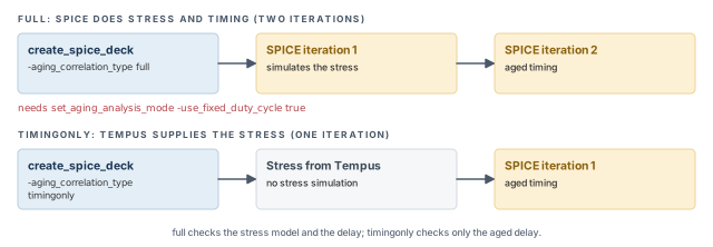
full– SPICE simulates both the stress and the timing, in two iterations. It needsset_aging_analysis_mode -use_fixed_duty_cycle true.timingonly– the tool supplies the stress, and SPICE runs one timing iteration.
timingonly checks only the delay calculation. full also checks the stress model, so it is the stronger but slower test. Figure 17 sets the two side by side.
7 Worked example: a two-domain block, signed off honestly
Let us join the pieces for one block. The assumptions are written as comments at the point of use.
The task. Block abc has two domains. PD1 runs at 0.7 V or 0.8 V, and PD2 at 0.9 V or 1.0 V. The power manager never runs PD1 at 0.8 V while PD2 is at 0.9 V. The block uses CPF, sits in a dense area, and goes into a ten-year product.
Step 1 – load and validate binding
We start with binding, because every later step depends on it.
tempus> read_mmmc abc.tcl                       ;# assuming views and RC corners inside
tempus> read_verilog abc.v                      ;# netlist
tempus> set_top_module abc                      ;# link
tempus> read_power_intent -cpf abc.cpf          ;# two domains
tempus> read_spef -rc_corner rc_wc abc.spef     ;# CPF has no RC corners
tempus> update_timing -full                     ;# first timing
tempus> report_instance_library pd1_inst/U7     ;# expect a PD1 library
tempus> report_instance_library pd2_inst/U9     ;# expect a PD2 library
What to look for. The library for U7 must belong to PD1's voltage, and U9's to PD2's. If either is wrong, stop and fix the CPF.
Step 2 – audit crossings, then define signatures
tempus> check_ipd_logic -multi_pd_type all \
          -outfile ipd_logic_check_report -verbose   ;# audit risky crossings
tempus> set_ipd_rail_voltage -sweep { PD1 {0.7 0.8} PD2 {0.9 1.0} } \
          -exclude_voltage_signatures { {PD1 0.8 PD2 0.9} }   ;# impossible combo
Assume the audit flags one clock path with three domains after its common point. We fix that clock path first, because it would multiply the corner count.
The sweep gives 2 × 2 = 4 signatures. One is excluded, so run 2 times the scoped paths at 3 signatures.
Step 3 – run the two IPD runs
Run 1 writes ipd_scope with write_ipd_scope. Run 2 reads it and reports with report_timing -ipd, exactly as in the IPD section.
What to look for. Compare the worst IPD slack with the bounded-corner slack. A worse result at the mixed signature (0.7 V / 1.0 V) confirms why IPD was needed.
Step 4 – add IR drop
The block has a dense area with high switching. We run Tempus PI and report with best average early and worst average late.
What to look for. Compare the IR-aware slack with the slack from Step 1 of this example, which had no IR drop. Paths that lose the most slack sit in hot spots. Those are the paths to fix in the IR-aware ECO.
Step 5 – add aging
The product has a ten-year life. We add a stress profile in a separate session, with aging on before the first update. We check aged slack on the paths that were already tight.
All voltages, names and the audit result are illustrative. They show the order of decisions, not real data.
8 Common mistakes and how to catch them
Table 6 gathers the mistakes from this chapter.
| Symptom | Likely cause | Fix |
|---|---|---|
| Clean multi-supply report, wrong in silicon | Instances bound to the wrong voltage library | Check report_instance_library and report_delay_calculation -voltage |
| Parasitics missing in a CPF run | CPF has no RC corners | Create RC corners and use read_spef -rc_corner |
| PGV MMMC run fails at view setup | set_analysis_view before infer_pgv_power_intent, or two active views |
Set one view, after inference |
| PGV binding has no effect | set_lib_binding_by_voltage before set_top_module |
Bind after linking |
| A CPF option has no effect | Option is not supported for timing | Check Table 3 |
| IPD run takes far too long | Stray path with many domains after the common point | Run check_ipd_logic and fix the path |
| IPD report shows non-crossing paths | Plain report_timing used |
Use report_timing -ipd |
| IR-aware slack equals the budget run | -irdrop_data points at the wrong folder |
Point it at the real rail output |
| IR values look clamped or noisy | Guard and check thresholds misunderstood | Check threshold 0.25 warns; guard threshold 1 clamps |
| Tempus PI power step fails | Method is not dynamic_vectorless |
Use -method dynamic_vectorless |
| UDCP has no effect | Set after report_power |
Set UDCP before report_power |
| Fresh timing impossible after aging run | Aging mode cannot be turned off | Run fresh timing in its own session |
full SPICE correlation fails |
Fixed duty cycle not set | Set -use_fixed_duty_cycle true |
9 Interview preparation
Less supply voltage gives less drive current, so the load charges more slowly.
- The output edge is both later and slower.
- The slower edge also slows the next cell, through its input slew.
That each instance is bound to the library for its domain's voltage.
- Use
report_instance_libraryandreport_delay_calculation -voltage. - Check cells on both sides of each level shifter, because that is where mistakes hide.
It infers them from the power-aware netlist: one domain per power net, named pd_<net>.
- One library set is built per domain, from an internal CPF 1.0e description.
- In the single-view flow,
set_lib_binding_by_voltagefollowsset_top_module. - In the MMMC flow,
set_analysis_viewfollowsinfer_pgv_power_intent.
One combination of voltages across all swept domains.
- Two domains with two voltages each give four signatures.
-exclude_voltage_signaturesremoves combinations that never occur.
Run 1 finds the crossing paths cheaply at two bounded corners; run 2 times only those paths at every signature.
- Timing the whole design at every signature would be far too slow.
- The scope folder carries paths, constraints and derates from run 1 to run 2.
When it crosses domains and the CPPR point is missing, changes transition, or is followed by a domain change.
- Before the common point, the shared part cancels out.
- Paths with two or more domains after the common point can explode the corner count.
EIV is the effective instance voltage from rail analysis; use worst average for late (setup) timing.
- Best average is used for early (hold) timing.
- It is an average in a window, not the single lowest point.
The -irdrop_data path probably does not point at the real rail output.
- The estimated worst factor is ignored once real EIV data loads, so results should change.
- Check the folder name that
analyze_railactually wrote.
-irDrop_value_check_threshold and -irDrop_value_guard_threshold?The check threshold (0.25) only warns with IMPDC-3280; the guard threshold (1) clamps the value.
- A warning asks you to inspect the value; a clamp changes it.
- Both are safety nets against bad rail data.
BTI depends on duty cycle under voltage and temperature; HCI depends on toggle rate.
- A net held high for years ages through BTI even if it never toggles.
- Both slow cells down over the product's life.
At a special net – the output of a multi-input cell on the clock, or a user-set net – or at an endpoint.
- A clock gate's output depends on its enable, so the input duty cycle no longer applies.
- Multi-input cells on data paths are not special nets.
Through the stress-profile scales, because TMI is not recovery-aware.
-recovery trueneeds OMI, URI or Liberate libraries.- The
-bti_*and-hci_*scales range from 0 to 1, default 1.
Chapter recap
Key takeaways
- Supply voltage, IR drop and aging all change cell delay, so each cell must be timed at its real voltage.
- Load power intent with CPF or a PGV netlist, then prove the binding before trusting slack.
- CPF has no RC corners, and some CPF options are ignored for timing.
- IPD times crossing paths at every voltage signature, using a scope-creation run and an analysis run.
- Tempus PI replaces a flat IR margin with a per-instance EIV; early and late settings beat generic ones.
- Aging needs fresh and aged libraries, power intent, a stress profile and activity, with aging turned on before the first update.
Command recap
| Command | Purpose |
|---|---|
read_power_intent -cpf, read_mmmc -cpf, read_power_domain -cpf |
Read CPF power intent |
set_lib_binding_by_voltage, infer_pgv_power_intent |
Bind libraries from a PGV netlist |
report_instance_library, report_delay_calculation -voltage |
Validate binding |
set_op_cond, set_timing_library |
Non-MMMC binding |
define_library_set -user_attributes, getCPFUserAttributes |
CPF user attributes |
set_ipd_rail_voltage, create_pg_net_group |
Define IPD sweeps and rail groups |
create_ipd_configuration, write_ipd_scope, read_ipd_scope |
Build and reuse the IPD scope |
check_ipd_logic, report_timing -ipd |
Audit and report IPD paths |
set_power_analysis_mode, set_rail_analysis_mode, analyze_rail |
Power and rail analysis for EIV |
update_delay_corner -irdrop_data, set_delay_cal_mode, set_irdrop_mode |
Use IR-drop data in timing |
set_analysis_mode -aging true |
Turn on aging; cannot be turned off later |
create_aging_stress_profile, set_aging_activity, set_aging_analysis_mode |
Aging setup |
create_spice_deck |
SPICE correlation for aging |
Compact glossary
| Term | Meaning |
|---|---|
| Power domain (PD) | A group of cells on one supply |
| Power intent | A description of domains, supplies and voltages (CPF, UPF/1801 or PGV) |
| PGV | A power-aware netlist from which the tool infers power intent |
| Binding | Choosing the library each instance is timed with |
| Level shifter | A cell that translates a signal between two supply levels |
| SMSC | Single mode, single corner – one view |
| IPD path | A path whose timing depends on more than one domain's voltage |
| Voltage signature | One combination of voltages across the swept domains |
| Bounded corners | All domains at high voltage (min) or all at low voltage (max) |
| IR drop | Supply sag caused by current through the grid resistance |
| EIV | Effective instance voltage: the supply one instance sees, averaged in a window |
| UDCP | User-defined critical paths given to power analysis |
| BTI | Bias temperature instability: aging from stress while on |
| HCI | Hot carrier injection: aging from switching |
| Duty cycle | Fraction of time a signal is high |
| Toggle rate | Number of switches per second |
| Stress profile | Segments of duration, voltage and temperature over the product's life |
Practical perspective
On a real low-power project, these checks often run at different stages. Binding validation and IPD audits come early, because they find setup errors cheaply. Tempus PI runs once the power grid is stable, since the rail data depends on it. Aging is usually a signoff-stage check for long-life products. Thus, plan them as separate sessions, each with its own clear question.
What comes next
We now time each cell at its real voltage, across domains and over its life. In the next chapter, Advanced Checks and Timing Debug, we look at more checks. These include multi-input switching, VT skew, DRV and cell EM. We will also meet the tools for debugging timing.