Chapter overview
A clean timing report is only as good as the model behind it. Some real effects are not in the basic model at all. For example, two inputs of a NAND gate can fall at the same moment. The output then rises faster than the library table says. A hold check that looked safe can fail on silicon.
Other effects are not about delay at all. A cell pin can wear out because it toggles too often with a heavy load. A signal can switch too slowly and break a design rule, even when its path has positive slack. These checks sit beside timing and are part of every signoff.
This chapter collects such advanced checks, plus the tools that make debug and long runs practical. We start with multi-input switching (MIS) and its fast derate form. Then we cover VT skew, design rule (DRV) reporting and cell electromigration (EM). Finally, we look at the timing debug GUI, multi-CPU runs and SPICE correlation.
Each topic is independent. Thus, you can read the sections in any order once you know the basics from the earlier chapters. However, MIS and AMIS-derate are best read together, because the second is a faster form of the first.
Learning objectives
- Explain why inputs that switch together speed up a gate, and why this is an early (hold) concern.
- Select a multi-input switching mode and tune it with the alignment factor and alignment mode.
- Describe what AMIS-derate changes and what it leaves untouched, and compute a tuned derate.
- Set up Vth groups and VT-skew derates, and read the VT-skew report columns.
- Predict which DRV limit applies, and write DRV reports with custom fields and CSV output.
- Run a cell EM check with switching activity, and verify the toggle rates behind it.
- Load reports into the timing debug GUI and sort failing paths into categories.
- Configure multi-CPU usage with licenses and measure the resources a command needs.
- Build a SPICE deck for a path and work through a miscorrelation checklist.
Chapter roadmap
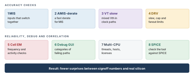
The chapter moves from accuracy checks to reliability, debug and correlation. Figure 1 shows the eight topics. Come back to it whenever you lose your place.
Key commands
Table 1 lists the main commands by section. Do not try to memorize them now. Each one is explained when it is first needed.
| Section | Command | What it does |
|---|---|---|
| 1 MIS | set_analysis_mode -multi_input_switching_mode |
Turns MIS off or picks one of its modes |
| 1 MIS | set_multi_input_switching_mode |
Tunes alignment and excludes cells |
| 2 AMIS-derate | report_delay_calculation -mis |
Shows the AMIS derate on one arc |
| 3 VT skew | set_threshold_voltage_group |
Groups library cells by threshold voltage |
| 3 VT skew | set_vt_skew_derate, set_vt_skew_config |
Sets the derates and limits the group pairs |
| 4 DRV | report_constraint -drv_violation_type |
Reports transition, capacitance and fanout violations |
| 5 Cell EM | propagate_activity -set_net_freq true |
Spreads switching activity and sets net frequencies |
| 5 Cell EM | report_freq_violation |
Reports frequency-based EM violations |
| 6 Debug GUI | load_timing_debug_report |
Loads a timing report into the GUI |
| 6 Debug GUI | create_path_category |
Groups paths into a named category |
| 7 Multi-CPU | set_multi_cpu_usage, report_resource |
Sets threads and licenses; measures run cost |
| 8 SPICE | create_spice_deck |
Writes, and optionally simulates, a SPICE deck for a path |
1 Multi-input switching (MIS)
1.1 The concept
A library delay table for a NAND gate assumes one input switches at a time. The other inputs sit at steady, non-controlling values. For a NAND gate, the non-controlling value is 1. Real circuits do not always behave so politely.
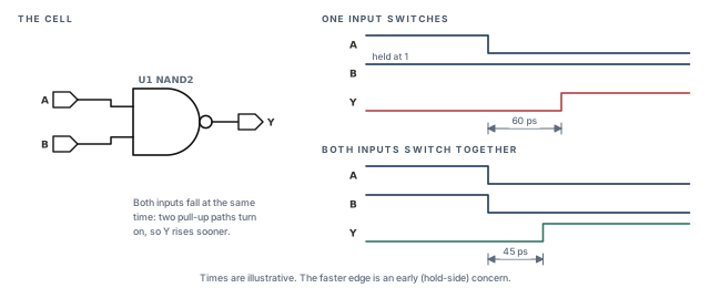
Let us look inside a NAND2 for a moment. Its output is pulled up by two PMOS transistors in parallel, one per input. When one input falls, one PMOS turns on and charges the output. When both inputs fall together, both PMOS transistors turn on. Two parallel paths deliver more current, so the output charges faster.
Let us consider the NAND2 cell U1 in Figure 2. When only A falls, Y rises after 60 ps. When A and B fall together, Y rises after 45 ps. The 15 ps difference is not in the library table, which only describes the single-input case.
This speed-up is called multi-input switching. The tool models it only as an early speed-up. In other words, it lowers early (minimum) delays and leaves late delays alone. It applies in both graph-based analysis (GBA) and path-based analysis (PBA). Inputs that are tied to the same net always switch at the same time, so the tool always treats them as simultaneous.
1.2 Why it matters
A hold check fails when data arrives too early at the capture flop. Every library delay on a hold path assumes one switching input. If two inputs really switch together, the true early delay is smaller. Thus, ignoring MIS can hide real hold violations.
A hold violation is worse than a setup violation. Setup failures can be fixed by slowing the clock. A hold failure breaks the chip at every clock speed. That is why MIS matters most during final hold signoff, where margins are only a few picoseconds.
1.3 Choosing the MIS mode
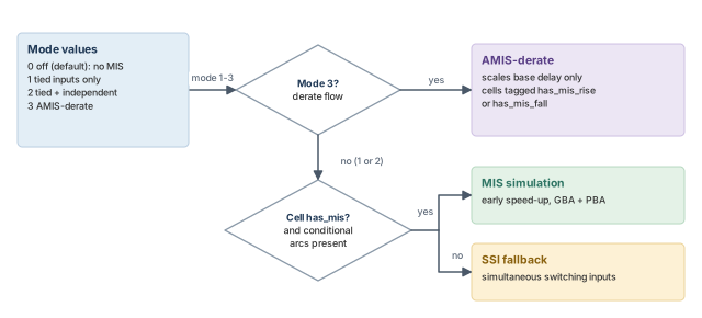
The main switch is an option of set_analysis_mode. It takes one of four integer values.
tempus> set_analysis_mode -multi_input_switching_mode 2 ;# tied + independent inputsTable 2 lists the four values. Modes 1 and 2 model more situations, at a higher runtime cost. Mode 3 trades some accuracy for speed.
| Value | Meaning | When you would use it |
|---|---|---|
0 |
MIS off (the default) | Early runs, or setup-only analysis |
1 |
Only tied inputs are treated as switching together | A cheap first look at the most certain cases |
2 |
Tied inputs and independent inputs | Full simulation-based hold signoff |
3 |
AMIS-derate, a fast derate-based form (Section 2) | Large designs where simulation is too slow |
- Mode 0 keeps the classic single-input model. It is the default, so MIS never turns on by accident.
- Mode 1 looks only at inputs driven by the same net. Their switching is certain, so this mode adds no guesswork.
- Mode 2 adds independent inputs, driven by different nets. Their switching times must be estimated, which the alignment options below control.
- Mode 3 replaces simulation with a derate. Section 2 covers it in detail.
1.4 Which cells get MIS
Not every cell takes part. A library cell is eligible only when its has_mis property is true. The library sets this property, not the designer. You can still leave out cells you do not trust, for example a cell whose data was never characterized for MIS:
tempus> set_multi_input_switching_mode -disable_lib_cells {lib1/NAND4X1} ;# skip this cellMIS also needs conditional arcs in the library. A conditional arc states the values of the other inputs, for example "A to Y when B is 1". In other words, the library must state which single-input case each table describes.
The tool then decides how to model each cell. Cells with has_mis and conditional arcs use MIS instead of simultaneous switching inputs (SSI) modeling. Other cells fall back to SSI, which Path-Based and Robustness Analysis covers. Figure 3 shows the full decision.
- A NOR3 cell's fall-to-rise transition is not modeled by MIS. SSI still applies to that transition.
- Thus, a missing MIS effect on such a cell is expected, not a setup error.
1.5 The alignment factor
In mode 2, the tool must decide when each other input switches. We call the input on the path being timed the main input. The others are side inputs. Each side input has a window of possible arrival times, from its early arrival to its late arrival.
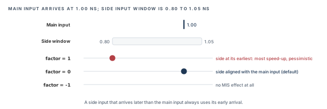
The -switching_alignment_factor option, from -1 to 1, places the side input inside its window. Let us consider Figure 4. The main input arrives at 1.00 ns. A side input can arrive anywhere from 0.80 to 1.05 ns.
- Factor 1 – the side input switches at its earliest arrival, 0.80 ns. This gives the most speed-up. It can even give negative delays, so it is the most pessimistic choice.
- Factor 0 (the default) – the side input is aligned with the main input, at 1.00 ns. Both edges overlap fully, which is the classic MIS picture.
- Factor -1 – no MIS effect at all. The cell behaves as if only the main input switched.
- Values in between – place the side input between these cases. For example, 0.5 lies between aligned and earliest.
One rule always holds. A side input that arrives later than the main input always uses its early arrival. This is the pessimistic choice for hold, because an earlier side edge gives more speed-up.
The -mis_alignment_mode option takes 0 or 1 and selects an overlap mode. In overlap mode, side inputs that arrive far earlier than the main input are treated as static. In other words, they have already settled, so they cannot speed up the main input. The flow script below sets it to 1. Confirm which value enables overlap mode with help set_multi_input_switching_mode.
tempus> set_multi_input_switching_mode -switching_alignment_factor 0.5   ;# halfway
tempus> set_multi_input_switching_mode -mis_alignment_mode 1 ;# overlap modeIt is better to start with the default factor of 0. A factor of 1 can create negative delays and many false hold violations. Raise it only if SPICE correlation shows that 0 is optimistic for your library.
1.6 Per-cell alignment factors
Sometimes one cell type needs its own factor. For example, a large NAND4 might correlate better with a different value than the rest of the library. The tool supports this through library-cell properties.
You define the properties inside interactive constraint mode, opened for all constraint modes. The rise and fall cases each have their own property, bounded from -1 to 1:
tempus> set_interactive_constraint_modes [all_constraint_modes]   ;# edit all modes
tempus> define_property -object_type lib_cell -type float mis_alignment_factor_min_rise \
          -lower_bound -1 -upper_bound 1                         ;# rise factor property
tempus> define_property -object_type lib_cell -type float mis_alignment_factor_min_fall \
          -lower_bound -1 -upper_bound 1                         ;# fall factor property
tempus> set_interactive_constraint_modes {}                       ;# leave interactive mode
The property is then given a value on the chosen library cells. Confirm the exact command for setting the value with help define_property in your installation.
The rise property name also appears spelled mis_alignments_factor_min_rise (with an extra "s"). Confirm the exact name with help before relying on it. A misspelled property is simply ignored, so the cell silently keeps the global factor.
1.7 How clocks affect simultaneity
Two inputs can only switch together if their clocks allow it. The tool uses the clock relationships from the constraints:
- Inputs on physically exclusive clocks are never simultaneous. Such clocks can never exist on the chip at the same time.
- Inputs on asynchronous clocks are treated as switching together. Their phase is unknown, so any overlap is possible.
- With
set_si_mode -use_infinite_TW true, all inputs that are not on physically exclusive clocks are treated as together. Infinite timing windows remove all timing separation.
Figure 5 shows the three cases on a NAND2 whose inputs come from two clock domains.
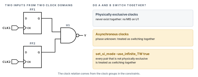
Thus, the clock groups you wrote for crosstalk also shape MIS. A wrong clock group can either hide MIS or add false MIS.
1.8 Reporting the MIS effect
The MIS change appears in a PBA retimed report through the retime_mis_delta field. A negative delta means the arc became faster because of MIS.
tempus> report_timing -format {retime_mis_delta} ;# PBA retime: MIS change per arcFor SPICE checks, MIS is supported at stage level only, with create_spice_deck -enable_mis. A full path deck does not include MIS. Section 8 covers SPICE decks.
1.9 The complete MIS setup
The full flow uses simulation-based delay calculation. The first four commands load the design. The next three commands raise delay-calculation accuracy, because MIS relies on waveform simulation. The last commands select MIS and retime the design.
read_view_definition viewDef.tcl                           ;# MMMC views
read_verilog netlist.v                                     ;# netlist
set_top_module top                                         ;# link
read_spef -rc_corner RC_worst design.spef ;# parasiticsset_delay_cal_mode -accuracy_level 3 ;# highest accuracy
set_delay_cal_mode -ewm_type simulation \
-equivalent_waveform_model propagation ;# simulated waveforms
set_delay_cal_mode -advanced_pincap_mode 2 ;# advanced pin cap
set_analysis_mode -multi_input_switching_mode 2 ;# tied + independent
set_multi_input_switching_mode -mis_alignment_mode 1 ;# overlap mode
set_multi_input_switching_mode -disable_lib_cells {lib1/NAND4X1} ;# optional
set_multi_input_switching_mode -switching_alignment_factor 0 ;# optional
update_timing -full ;# full timing update2 AMIS-derate: a faster MIS
2.1 The concept
Full MIS simulates each multi-input cell, which costs runtime on a large design. AMIS-derate is a lighter form. Instead of simulating, it multiplies the base delay by a derate below 1. A derate of 0.90 makes the arc 10% faster.
Set mode 3 to use it. Mode 3 automatically disables simulation-based AMIS, so the two never run together. You can still leave out cells you do not trust:
tempus> set_analysis_mode -multi_input_switching_mode 3   ;# AMIS-derate
tempus> set_multi_input_switching_mode \
          -disable_lib_cell {lib1/AOI22X1}                 ;# optional exclusion
Note the option spelling here: -disable_lib_cell, without the final "s". Eligible cells carry the tags has_mis_fall or has_mis_rise. As the names suggest, each tag marks one transition direction.
2.2 What the derate touches
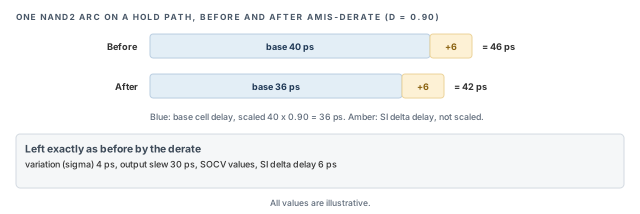
The derate is deliberately narrow. It changes only one number on each eligible arc. Table 3 lists what it changes and what it leaves alone.
A simple way to remember the rule: the derate scales only the nominal delay. Every other effect keeps its own model, so sigma, crosstalk and slew are reported exactly as before.
| Changed | Not changed |
|---|---|
| Base cell delay | Variation (sigma), SI delta delay, slew, and any SOCV values |
Figure 6 applies this rule to one arc. The base delay of 40 ps is scaled by 0.90. The 6 ps crosstalk delta and the sigma stay as they were.
2.3 How the derate is chosen
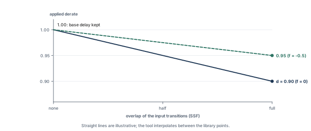
The derate is not a fixed number. It depends on how much the input transitions overlap. In outline, full overlap gives the full derate, and little overlap leaves the derate near 1. The tool interpolates between these cases using an overlap measure it labels SSF.
Figure 7 shows this interpolation for a library derate of 0.90. Clock groups are ignored in this mode, unlike in simulation-based MIS. SSI can coexist with AMIS-derate. Where a cell supports AMIS-derate, the AMIS-derate wins.
2.4 The alignment factor in derate mode
In derate mode, -switching_alignment_factor runs from 0 to -1. It softens the derate. Let d be the derate and f the factor. The tuned derate is:
tuned = d - (1 - d) x fLet us work through three cases by hand. All use d = 0.90.
- With f = 0, tuned = 0.90 − (0.10 × 0) = 0.90. The full derate applies.
- With f = −0.5, tuned = 0.90 − (0.10 × −0.5) = 0.90 + 0.05 = 0.95.
- With f = −1, tuned = 0.90 + 0.10 = 1.00. The derate disappears, so there is no MIS effect.
Thus, a negative factor moves the derate toward 1, which means less speed-up. The per-cell properties mis_alignment_factor_min_rise and _fall take bounds from -1 to 0 in this mode.
2.5 Reporting
The derate column appears in PBA retimed reports. The report header shows AMIS, so you can see at a glance that the derate was active.
# PBA only: the derate column appears after retiming
tempus> report_timing -early -retime path_slew_propagation \
          -format {instance arc cell retime_delay retime_slew retime_mis_derate arrival}
tempus> report_delay_calculation -from i0/i1 -to i0/o -min -mis ;# derate on one arcreport_timingwithretime_mis_deratein-formatshows the derate on every arc of the retimed path.report_delay_calculation -misexplains the derate on a single arc. Use it when one cell looks suspicious.
3 VT skew
3.1 The concept
Cells come in threshold voltage (Vth) flavors. Low-Vth (LVT) cells are fast but leaky. High-Vth (HVT) cells are slow but save power. Many designs mix them, even in clock trees.
Process variation does not move every flavor by the same amount. For example, on one die LVT cells may come out 4% fast while HVT cells come out 2% slow. If the launch and capture clock paths use different flavors, they drift apart. The clock skew on silicon then differs from the skew in the report.
3.2 Why it matters
Without this feature, a team would typically add a flat guard-band for mixed-Vth clock paths. A flat margin is too pessimistic for paths that use one flavor, and may be too small for badly mixed ones. VT-skew derates apply margin only where the flavors really differ.
3.3 How the derate is placed
Let us consider Figure 8. After the CPPR point, the launch branch uses LVT buffers and the capture branch uses HVT buffers. The common part before the CPPR point is shared, so it cannot cause skew. Only the two branches matter. The tool applies a VT-skew derate to capture this risk.
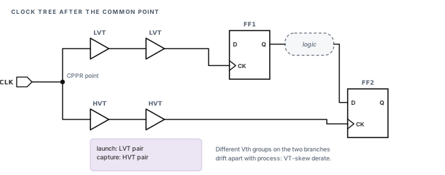
3.4 Setting it up
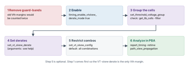
Setup follows four steps:
- Remove any existing Vth guard-bands. Otherwise the same risk is counted twice and hold or setup slack becomes falsely negative.
- Enable the feature with the global
timing_enable_vtskew_derate_mode. - Group the library cells by threshold voltage with
set_threshold_voltage_group, and check the membership. - Set the derates with
set_vt_skew_derate, and optionally restrict the combinations withset_vt_skew_config.
tempus> set timing_enable_vtskew_derate_mode true                     ;# enable the feature
tempus> set_threshold_voltage_group -name LVT \
          -lib_cells [get_lib_cells *_lvt*/*]                         ;# LVT group
tempus> get_lib_cells */* -filter {threshold_voltage_group == "LVT"}  ;# check membership
tempus> set_vt_skew_config -unique_vt_mode slow ;# unique-Vt modeset_threshold_voltage_group– names a group and lists its library cells. Repeat it for each flavor, such as SVT and HVT. A cell left out of every group cannot be derated correctly.get_lib_cells -filter– lists the cells now in a group. Use it to catch a wildcard that matched too much or too little.set_vt_skew_derate– sets the derate values for the group combinations. Its arguments are not shown here; check them withhelp set_vt_skew_deratebefore writing the script.set_vt_skew_config– restricts which group combinations are derated. By default, all combinations are. The-unique_vt_mode slowsetting selects the unique-Vt mode described below.
Figure 9 shows the whole order, from removing old margins to the PBA report.
3.5 How the analysis runs
VT-skew analysis runs in PBA, because the derate depends on the exact cells on each path. In unique-Vt mode, the clock cells after the CPPR point must be in the same Vth class. This mode can be used with -max_slack greater than 0, so near-critical paths are checked too.
The report adds three columns: vt_group, vt_skew_derate and total_derate. As the names suggest, they show each cell's group, the VT-skew derate on the arc and the overall derate. Confirm the exact column meanings with help report_timing.
For a per-combination table on a path, add the debug option:
tempus> report_timing -retime path_slew_propagation -debug vt_skew ;# slow: use on few pathsThe debug table is slow. It is better to run it on a handful of paths you already suspect, not on the whole design.
4 DRV reporting
4.1 The concept
Design rule violations (DRV) are broken limits on transition, capacitance and fanout. They protect signal quality and reliability, not timing directly. For example, a very slow transition makes a gate burn short-circuit current and pick up more noise.
A path can have positive slack and still break a design rule. Thus, signoff checks both timing and DRV. This section covers how to read and shape DRV reports.
4.2 Which limit applies
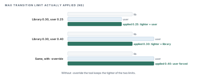
A limit can come from the library or from the user. By default, the tool uses the tighter of the two. This protects you when a library limit is stricter than your constraint.
Sometimes you want a looser user limit on purpose, for example after a waiver from the library team. The -override option forces the user value. It works on set_max_transition, set_min_transition, set_max_capacitance, set_min_capacitance, set_max_fanout and set_min_fanout.
Figure 10 shows three cases for max transition:
- Library 0.30 ns, user 0.25 ns: the user value is tighter, so 0.25 ns applies.
- Library 0.30 ns, user 0.40 ns: the library value is tighter, so 0.30 ns applies.
- The same values with
-override: the user value 0.40 ns applies.
4.3 Violation types
The tool knows eight DRV types. Each name says what is limited and in which direction:
max_transitionandmin_transition– slowest and fastest allowed transition.max_capacitanceandmin_capacitance– largest and smallest allowed load.max_fanoutandmin_fanout– largest and smallest allowed fanout.pulse_clock_max_transitionandpulse_clock_min_transition– transition limits on pulse clocks.
4.4 Reporting
The main command is report_constraint. You choose the types, the fields and the output format.
tempus> report_constraint -drv_violation_type {max_transition max_capacitance}   ;# two types
tempus> set timing_report_constraint_format {pin ref_cell transition_slack}   ;# fields
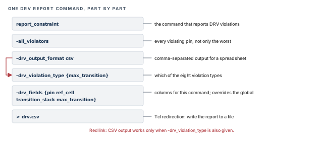
tempus> report_constraint -all_violators -drv_output_format csv \
          -drv_violation_type {max_transition} \
          -drv_fields {pin ref_cell transition_slack max_transition} > drv.csv    ;# CSV file
Figure 11, after the list below, takes the CSV command apart, one option per row.
The options work as follows:
-drv_violation_type– selects one or more of the eight types. CSV output is possible only when it is given.timing_report_constraint_format– a global that lists the fields to print. It defaults to{}, which means the classic format.-drv_fields– lists fields for one command and overrides the global. Fields that do not fit a violation type are ignored, not reported as errors.-drv_output_format csv– writes comma-separated output for a spreadsheet. It works only together with-drv_violation_type.-all_violators– lists every violating pin, not only the worst.-worst_drv_per_net– keeps only the worst violation on each net, which shortens long reports.-max_pins_per_drv N– limits the pins printed per violation.-clockand-data– keep only clock nets or only data nets.
For text reports, set_table_style -no_frame -nosplit prints tables without frames and without split rows. This helps when a script parses the report.
4.5 Across views and run styles
- In concurrent MMMC, set
timing_report_drv_use_worst_timing_slacktotrue. The report then shows the worst value across all views. - In distributed STA,
-worst_drv_per_netand the fieldstransition_si,max_slackandmin_slackare not supported. - In distributed MMMC, DRV reports cannot be merged with
merge_timing_reports. Keep the per-view reports instead. - DRV reporting is not used for cell EM. Section 5 covers that check.
A beginner relaxes the max transition to 0.40 ns and expects fewer violations. None disappear, because the tighter 0.30 ns library limit still applies. Add -override only when the looser limit is truly approved.
5 Cell electromigration (EM)
5.1 The concept
Current flowing through a metal wire slowly pushes metal atoms along. Over years, this electromigration can thin a wire until it opens. Inside a cell, the risk typically sits on the output pin connection, which carries the charging current of the load.
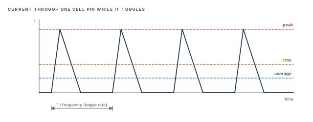
The current depends on three things: the load capacitance, the transition time and the toggle frequency. A pin that switches twice as often carries twice the average current. Thus, cell EM is a frequency check, not a timing check.
Figure 12 shows the current through one pin while it toggles. A limit can be on the average, the root-mean-square (rms) or the peak current. By default, the tool checks the worst of the three.
5.2 Why it matters
An EM failure does not show up at test. The chip works for months, then a pin opens in the field. A missed EM violation is therefore a reliability failure, not a yield loss. On the other hand, a false violation wastes ECO effort on cells that were never at risk.
5.3 Which view is checked
Set the EM view with set_analysis_view -dynamic <view>. Without it, the tool uses the first setup view. That fallback is tied to the check type set with set_analysis_mode -checkType. Thus, it is better to name the EM view explicitly, so the result does not depend on view order.
5.4 Library data
The tool looks for EM limits in the library, in this order of preference:
- A
max_captable indexed by frequency and slew, built from amaxcap_lut_template. This form is preferred, and it states the allowed load directly. - Otherwise,
electromigrationdata withem_max_toggle_ratefor average, peak or rms current. That table uses anem_lut_template, and the tool reads it by reverse lookup.
Without EM libraries, set the limits yourself with set_max_cap_per_freq and set_max_tran_per_freq. However, report_freq_violation does not work in that case. Use report_constraint instead.
5.5 Switching activity
Frequency comes from switching activity – how often each net toggles. Several sources can set it. Table 4 lists them, highest priority first. A higher source always overrides a lower one on the same object.
| Priority | Source | Typical use |
|---|---|---|
| 1 (highest) | set_switching_activity |
Hand-set values for a few known nets |
| 2 | read_activity_file (VCD, TCF, FSDB, PHY or SAIF) |
Activity from simulation |
| 3 | Constants from the SDC | Pins tied by case analysis |
| 4 | set_default_switching_activity |
Defaults for everything else |
| 5 (lowest) | propagate_activity |
Values spread through the logic |
For example, assume a net gets 0.3 from a VCD file and 0.1 from set_switching_activity. The tool uses 0.1, because the user command has the higher priority.
Figure 13 shows the same ladder next to this example.
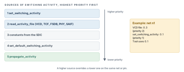
propagate_activity has the lowest priority, so any other source on the same net wins.5.6 The cell EM flow
Figure 14 shows the order of the steps. The order matters: some globals must be set before the libraries are read, and some commands only work after timing is updated.
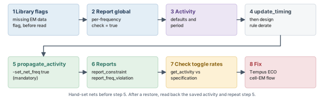
set timing_library_flag_cell_missing_em_data 1      ;# default 0; set before reading libraries
set timing_report_drv_per_frequency_per_input_slew true   ;# required; default false
set_default_switching_activity -black_box_density 0 -black_box_duty 0 \
    -seq_activity 0.2 -clock_gates_output 2.0         ;# default activities
set_default_switching_activity -period 2.0            ;# activity period
set timing_report_default_frequency_for_unconstrained_nets 2   ;# default 1e9
update_timing                                         ;# timing first
set_design_rule_derate [get_lib_pins *] 1.5           ;# after update_timing
propagate_activity -set_net_freq true                 ;# mandatory; works in DSTA too
report_constraint -drv_violation_type max_capacitance -all_violators   ;# EM cap check
report_constraint -check_type electromigration -all_violators -verbose ;# EM detail
report_freq_violation -reportFormat 1 -slew max       ;# writes freqViolation.rpt
Let us walk through the important lines:
timing_library_flag_cell_missing_em_data– flags cells without EM data with message TECHLIB-1260. It defaults to 0 and must be set before the libraries are read, because the check happens during reading.timing_report_drv_per_frequency_per_input_slew– must betruefor the frequency-based check. It defaults tofalse, so forgetting it silently skips the check.set_default_switching_activity– sets activity for objects with no other source. The example sets black-box density and duty to 0, sequential activity to 0.2 and clock-gate output activity to 2.0.-periodsets the period the activities refer to.timing_report_default_frequency_for_unconstrained_nets– the frequency used for nets with no clock. Its default is 1e9; the example sets 2. Confirm the unit withhelpbefore choosing a value.set_design_rule_derate– applies a factor to the design rule limits of the listed library pins. It must come afterupdate_timing.set_switching_activity– if you hand-set any nets, do it beforepropagate_activity, so the propagation starts from your values.propagate_activity -set_net_freq true– spreads activity through the logic and writes net frequencies. It is mandatory, and it also works in distributed STA.report_freq_violation– takes-reportFormat 1or2, and an optional-slew max. It writesfreqViolation.rpt.
Three more globals handle lookups that fall outside the library tables. All default to false:
timing_library_em_cap_lookup_slew_out_of_bounds– clamps a slew that falls outside the table.timing_library_handle_out_of_bound_frequency– clips a frequency that falls outside the table.timing_report_enable_em_index_clipping_report– marks clipped lookups in the report as(Tr OB)or(Ld OB).
To check the activity on any object, use get_activity -pin, -port or -net.
Propagated activity is not saved with the design. Before saving, write it with write_tcf. After a restore, read it with read_activity_file, and always rerun propagate_activity.
5.7 Hierarchical flows
Hierarchical designs need the block to see the right activity at its ports:
- For multiple instances of one module (MIM), set
set_power_analysis_mode -worst_case_vector_activity true. Each port then gets the worst activity of all instances. - With a timing context, write it at the top with
write_timing_context context.db -module block -include_TCF. The activity travels inside the context. - At the block, read it with
read_timing_context context.db -tcf_port_type data|clock|both. The default isdata. Then runupdate_timingandpropagate_activity -set_net_freq true. - With boundary models, use
create_boundary_model -dir DIR -include_TCFandread_boundary_model DIR -module block, where-modulenames the block.
Always compare the reported toggle rates with the design specification before you trust an EM violation. A wrong default activity can create hundreds of false violations. Real fixes then go through the Tempus ECO cell-EM flow, covered in Signoff ECO.
6 The timing debug GUI
6.1 The concept
A report with 5,000 failing paths is hard to read as text. Often most of them share one cause, such as one slow clock buffer or one missing exception. The timing debug GUI groups paths so you can see those patterns.
The GUI works offline, so you can debug saved reports without keeping the timing session open. This typically frees licenses and memory. The GUI loads gtd.pref.tcl automatically at startup, so personal settings can live in that file.
Figure 15, after the next list, shows the flow from report to categories.
6.2 Writing and loading reports
report_timing -machine_readablewrites an.mtarptfile, the machine-readable form the GUI loads. In the GUI, the default is-max_points 10000 -max_slack 0.75.write_text_timing_reportis the other way to write a report for the GUI.load_timing_debug_reportloads a report into the GUI. With Append, each report is colored separately, so two runs can be compared.
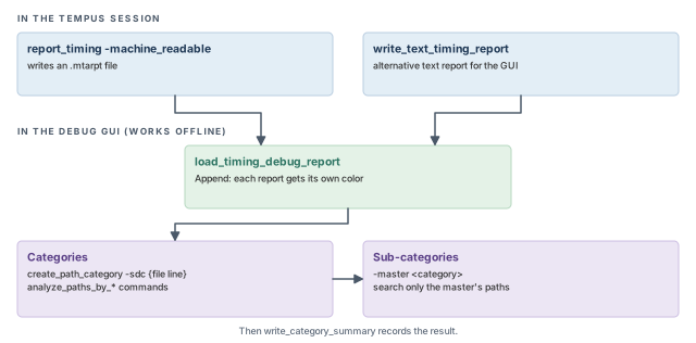
6.3 Path categories
A category is a named group of paths. You can create one from SDC lines. This shows which paths a particular constraint line affects:
tempus> create_path_category -name io_paths -sdc {top.sdc 120}   ;# from line 120
tempus> create_path_category -name io_slow -master io_paths \
          -sdc {top.sdc 121}                                    ;# sub-category
tempus> write_category_summary ;# summary-name– the category name shown in the GUI.-sdc {file line}– the constraint line that defines the category.-master <category>– makes a sub-category inside an existing category.
The tool also builds categories automatically. The commands are analyze_paths_by_basic_path_group, analyze_paths_by_bottleneck, analyze_paths_by_clock_domain, analyze_paths_by_critical_false_path, analyze_paths_by_drv, analyze_paths_by_hierarchy and analyze_paths_by_view. Each name says how the paths are grouped. For example, as its name suggests, the bottleneck form looks for cells shared by many failing paths.
Note these rules:
- A sub-category searches only its master's paths.
- Deleting a parent category freezes its children. In other words, the children stop following changes to the parent.
- Slack corrections from several categories add up. A path in two categories gets both corrections.
- The Path SDC tab does not work for MMMC views.
- A custom column is a Tcl procedure with the arguments
{id var}. Source the procedure first, then add the column.
A beginner applies a 30 ps correction in one category and a 20 ps correction in another. A path in both categories gains 50 ps, not 30 ps. Check category overlap before trusting corrected slack.
7 Multi-CPU runs
7.1 The concept
Large designs need many CPUs to finish overnight. More CPUs need more licenses, as Getting Started with Tempus explained. This section shows how to request both, and how to measure what a command really costs.
tempus> set_distribute_host -local                                  ;# run on this machine
tempus> get_distribute_host                                         ;# check hosts
tempus> set_multi_cpu_usage -localCpu 4 \
          -licenseList {tempusl cndc tempusxl edsl edsxl} \
          -keepLicense true -threadInfo 1                           ;# 4 threads
tempus> check_multi_cpu_usage                                       ;# show setting
7.2 Command breakdown
set_distribute_host– says where work may run.-localkeeps it on this machine.get_distribute_hostshows the current setting.-localCpu– the number of local threads. Ask for no more than the machine has.-licenseList– the licenses the tool may use for extra CPUs.-keepLicense true– keeps the licenses checked out after use.-releaseLicensefrees them early instead, which helps other users on a shared license pool.-threadInfo– controls thread messages.0is the default,1prints a final summary, and2prints per-thread detail.check_multi_cpu_usage– prints the current settings, so you can confirm them in the log.
If you request more threads than the machine has, the tool prints a warning. A distributed run waits until all hosts are available, so one busy host delays the whole run.
7.3 Measuring resource use
Before a large batch, you need to know how much memory to reserve on the compute farm. report_resource measures one command between a start and an end marker:
tempus> report_resource -start report_timing          ;# start measuring
tempus> report_timing                                 ;# the command being measured
tempus> report_resource -end report_timing -verbose   ;# -verbose only with -end
The -verbose option is accepted only with -end. It prints the full breakdown for the measured command.
Figure 16 shows what the two markers capture during one run.
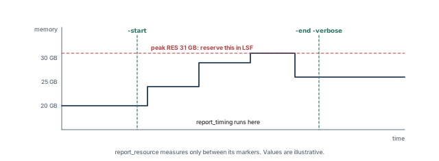
-start and -end is measured; its peak resident memory is the farm reservation (illustrative values).What to notice: Memory rises in steps while the command runs. The peak, not the final value, sets the reservation.The peak resident memory (RES) from report_resource is the value to reserve in LSF. Reserving less risks a killed job; reserving far more wastes the farm.
8 SPICE correlation
8.1 The concept
STA uses tables and models. SPICE simulates the actual transistors. When a critical path is in doubt, we simulate it in SPICE and compare the two. This is called SPICE correlation.
A good correlation gives confidence in the whole library and flow. A poor one usually points at a setup difference, not a tool error. Figure 17 shows the flow and the checks to run when the numbers disagree.
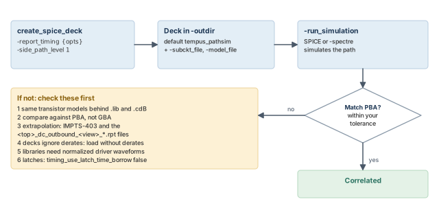
8.2 Command breakdown
create_spice_deck writes a deck for one path. Its options are:
-report_timing {opts}– picks the path with normalreport_timingoptions. Without it, the worst path is used. Add-path_type full_clockto include the clock path.-run_simulation(also spelled-run_path_simulation) – runs the simulation as well as writing the deck.-subckt_file– the transistor subcircuits for the cells.-model_fileis then required, because subcircuits need device models.-spectre– writes the deck for Spectre.-spice_includeadds include files to the deck. Confirm their exact effect withhelp create_spice_deck.-outdir– the output folder. The default istempus_pathsim.-side_path_level– from 0 (default) to 4. It adds side paths that load the main path. A value of 1 is recommended; higher levels make the deck larger and slower to simulate.-powerand-ground– the supply nets for the deck.-xtalk {delay|vl_glitch|vh_glitch}with-receiver_pin– a crosstalk deck for a single net. Path-level crosstalk is not supported.
tempus> create_spice_deck \
          -report_timing {-path_type full_clock -late -retime path_slew_propagation} \
          -run_simulation -side_path_level 1 -outdir tempus_pathsim   ;# deck + simulation
8.3 When the numbers disagree
Work through these causes in order. Each one is a setup difference that SPICE cannot see:
- Models – the
.liband the.cdBmust come from the same transistor models as the deck. - Analysis type – compare against PBA results. GBA is pessimistic by design.
- Extrapolation – look for message IMPTS-403 and the
<top>_dc_outbound_<view>_*.rptfiles. Values outside a table are extrapolated and less accurate. - Derates – decks ignore derates. Load the design without derates for a fair comparison.
- Driver waveform – the libraries need a normalized driver waveform (NDW).
- Latches – set
timing_use_latch_time_borrowtofalse, so borrowing does not change the compared arrival.
For example, assume Tempus PBA reports 410 ps and SPICE gives 395 ps. If OCV derates of 1.04 were on, the PBA delay without derates is 410 / 1.04, about 394 ps. Thus, the gap was the derate, not the delay model.
9 Worked example: a hold and EM signoff pass
Let us apply the chapter to one block. The assumptions are written as comments at the point of use.
The task. A 500 MHz block passes hold in GBA by 8 ps. The team asks for an MIS hold check, a DRV report for review, and a cell EM check. The design and views are already loaded.
Step 1 – turn on MIS for hold
We raise delay-calculation accuracy first, because MIS needs simulated waveforms. Then we select mode 2, so independent inputs are included.
# Assuming the design and views are already loaded (see Design Import)
set_delay_cal_mode -accuracy_level 3                       ;# accurate delay calculation
set_delay_cal_mode -ewm_type simulation \
    -equivalent_waveform_model propagation                 ;# simulated waveforms
set_delay_cal_mode -advanced_pincap_mode 2                 ;# advanced pin cap
set_analysis_mode -multi_input_switching_mode 2            ;# tied + independent
set_multi_input_switching_mode -mis_alignment_mode 1       ;# overlap mode
update_timing -full                                        ;# retime the design
report_timing -early -retime path_slew_propagation \
    -format {retime_mis_delta}                             ;# MIS deltas per arc
What to look for. Assume the worst hold path now shows an MIS delta of −11 ps on a NAND2. Assume also that its PBA slack before MIS was the same 8 ps. Thus, the margin becomes 8 − 11 = −3 ps. This is a real violation that GBA alone missed. Note which cell caused it, because Step 4 correlates it.
Step 2 – a DRV report for review
The review team wants a spreadsheet, so we write CSV. The type list is required for CSV output.
report_constraint -all_violators -drv_output_format csv \
    -drv_violation_type {max_transition} \
    -drv_fields {pin ref_cell transition_slack max_transition} > drv.csv   ;# CSV
What to look for. Sort by transition_slack. If many violations share one ref_cell, the cell may simply be too weak for its load.
Step 3 – cell EM
The clock runs at 500 MHz, so the period is 2.0 ns. We set the required global, give default activity and propagate it.
# Assuming the clock period is 2.0 ns (500 MHz)
set timing_report_drv_per_frequency_per_input_slew true    ;# required
set_default_switching_activity -seq_activity 0.2           ;# default flop activity
set_default_switching_activity -period 2.0                 ;# activity period
propagate_activity -set_net_freq true                      ;# mandatory
get_activity -net {n_bus[3]}                               ;# sanity check one net
report_freq_violation -reportFormat 1                      ;# writes freqViolation.rpt
What to look for. The braces around n_bus[3] stop Tcl from treating [3] as a command. Compare the reported activity on that net with what the designer expects. If it is far off, fix the activity before reading any violation.
Step 4 – verify before trusting anything
- Check that the activity on a few known nets matches the specification.
- Correlate the failing MIS hold path. Because MIS decks are stage-level only, use
create_spice_deck -enable_mison the NAND2 stage, and compare with PBA. - Write the activity with
write_tcfbefore saving the session, so a restore can read it back.
10 Common mistakes and how to catch them
Table 5 collects the mistakes from this chapter. Each row gives the symptom you would see first.
| Symptom | Likely cause | Fix |
|---|---|---|
| Hold passes in STA, fails on silicon | MIS off (mode 0 is the default) | Set mode 1, 2 or 3 and recheck hold |
| A cell gets no MIS effect | No has_mis, no conditional arcs, or NOR3 fall-to-rise |
Expect SSI instead; check the library |
| Negative delays appear | Alignment factor 1 (side input at earliest) | Use 0 unless you need the pessimism |
| Per-cell factor ignored | Property name misspelled | Check the name with help |
| AMIS speed-up smaller than expected | Negative alignment factor softening it | Check the factor; −1 removes the effect |
| VT-skew margin too large | Old Vth guard-bands still applied | Remove them before enabling VT skew |
| Looser user DRV limit has no effect | Tighter library limit wins | Add -override if approved |
| CSV DRV report not written | -drv_violation_type missing |
Add it; CSV needs it |
| No frequency-based EM results | Per-frequency report global left false | Set it to true |
| Hundreds of EM violations | Wrong default activity or frequency | Check get_activity and the toggle rates |
report_freq_violation does nothing |
No EM library data | Use report_constraint instead |
| EM results change after restore | Propagated activity not saved | Save with write_tcf; read back, propagate |
| Category slack looks too optimistic | Corrections from several categories added | Review overlapping categories |
| LSF job killed for memory | Reservation below peak RES | Reserve the measured peak |
| SPICE and STA disagree | Different models, GBA compared, or derates on | Work through the six checks |
11 Interview preparation
It is the speed-up of a gate when several inputs switch together; a faster gate threatens hold.
- The library table assumes one switching input, so it misses the extra drive current.
- The tool models MIS as early speed-up only, so only early delays change.
- Hold failures cannot be fixed by slowing the clock, which makes them costly.
-multi_input_switching_mode, and what do 1, 2 and 3 mean?The default is 0 (off). 1 is tied inputs only, 2 is tied plus independent inputs, and 3 is AMIS-derate.
- Modes 1 and 2 use simulation; mode 3 uses a derate and disables simulation-based AMIS.
- Each higher mode models more cases at more runtime, except mode 3, which trades accuracy for speed.
-switching_alignment_factor 1 do, and why is it pessimistic?It places the side input at its earliest arrival, giving the most speed-up, even negative delays.
- 0 (default) aligns the side input with the main input; -1 removes MIS.
- A side input later than the main input always uses its early arrival.
- The most speed-up means the smallest early delay, which is worst for hold.
has_mis property. Is it ignored for simultaneous switching?No. It falls back to SSI modeling.
- MIS also needs conditional arcs in the library.
- A NOR3 fall-to-rise transition is not modeled by MIS either, but SSI still applies.
It changes only the base delay; variation, SI delta, slew and SOCV values are untouched.
- The derate is interpolated by input overlap, and clock groups are ignored.
- Where a cell supports it, AMIS-derate wins over SSI.
0.95, from tuned = d − (1 − d) × f = 0.90 − 0.10 × (−0.5).
- A negative factor moves the derate toward 1, so the speed-up is halved here.
- A factor of −1 would give 1.00, which removes the effect.
Physically exclusive clocks never switch together; asynchronous clocks are treated as together.
- With infinite timing windows, all inputs not on physically exclusive clocks are together.
- Thus, the clock groups written for crosstalk also shape MIS results.
Remove any existing Vth guard-bands, so the margin is not counted twice.
- Then group cells with
set_threshold_voltage_groupand check membership withget_lib_cells -filter. - The analysis runs in PBA, because the derate depends on the cells on each path.
0.30 ns, the tighter one, unless you add -override.
- The rule protects you from relaxing a library limit by accident.
- With
-override, the 0.40 ns user value applies.
The switching activity and toggle rates, with get_activity, against the specification.
- Also check the default frequency for unconstrained nets, whose default is 1e9.
- Confirm that
propagate_activity -set_net_freq trueran after any hand-set activity.
propagate_activity after restoring a session?Propagated activity is not saved with the design.
- Write it with
write_tcfbefore saving. - Read it back with
read_activity_file, then propagate again.
Different transistor models behind the .lib and .cdB, comparing against GBA instead of PBA, and derates left on.
- Also extrapolation (IMPTS-403), missing NDW, and latch time borrowing.
- Each is a setup difference, so clear them before suspecting the tool.
Wrap it with report_resource -start and report_resource -end -verbose, and use the peak RES.
-verboseis accepted only with-end.- Reserving below the peak risks a killed job.
Chapter recap
Key takeaways
- MIS models the early speed-up of inputs switching together. It is off by default and matters for hold.
- The alignment factor sets how early side inputs switch. Factor 1 is the most pessimistic.
- AMIS-derate changes only the base delay, interpolated by overlap, and it wins over SSI where supported.
- VT skew derates mixed Vth groups after the CPPR point. Remove old guard-bands first.
- DRV limits use the tighter of library and user values unless
-overrideis given. - Cell EM depends on activity. Check toggle rates, and save activity with
write_tcf. - The debug GUI sorts paths into categories offline. Slack corrections from several categories add.
- Size farm jobs from the peak RES, and correlate doubtful paths against SPICE using PBA.
Command recap
| Command | Purpose |
|---|---|
set_analysis_mode -multi_input_switching_mode |
Choose MIS mode 0 to 3 |
set_multi_input_switching_mode |
Alignment factor, alignment mode, cell exclusion |
report_timing -format {retime_mis_delta} |
Show the MIS delta in PBA |
report_delay_calculation -mis |
Show the AMIS derate on an arc |
set_threshold_voltage_group, set_vt_skew_derate, set_vt_skew_config |
VT-skew setup |
report_timing -debug vt_skew |
Per-combination VT-skew table |
report_constraint -drv_violation_type, -drv_fields, -drv_output_format csv |
DRV reports |
set_default_switching_activity, set_switching_activity |
Default and user activity |
propagate_activity -set_net_freq true |
Propagate activity for EM |
report_freq_violation |
Frequency-based EM report |
get_activity, write_tcf, read_activity_file |
Check, save and restore activity |
load_timing_debug_report, create_path_category, write_category_summary |
Debug GUI |
set_multi_cpu_usage, check_multi_cpu_usage, report_resource |
Multi-CPU control and measurement |
create_spice_deck |
SPICE deck and simulation for a path |
Compact glossary
| Term | Meaning |
|---|---|
| MIS | Multi-input switching: several inputs of one gate switching together |
| SSI | Simultaneous switching inputs: the fallback model for cells without MIS data |
| AMIS-derate | A derate on base delay that stands in for MIS simulation |
| Main input / side input | The input on the timed path / the other inputs of the same gate |
| Conditional arc | A library arc that states the values of the other inputs |
| VT skew | Timing difference from different Vth groups on launch and capture clock paths |
| DRV | Design rule violation: transition, capacitance or fanout limit broken |
| Cell EM | Electromigration risk in a cell pin, driven by current and frequency |
| Toggle rate | How often a net switches per unit time |
| NDW | Normalized driver waveform in the library |
| EIV | Effective instance voltage: the supply voltage an instance actually sees |
| SMSC | Single mode single corner: one view per session |
| Startpoint | Where a timing path launches, such as a flop clock pin or input port |
| Endpoint | Where a timing path is captured, such as a flop data pin or output port |
Practical perspective
On a real project, these checks are not run every night. MIS and VT skew usually join the final hold signoff. Cell EM runs once the activity is trusted. The debug GUI and SPICE correlation are your tools when a result looks wrong. Thus, knowing they exist, and their traps, saves days when the deadline is close.
What comes next
So far, every analysis has run in one session on one machine or a few threads. In the next chapter, Distributed STA, we split a single large analysis across many machines and see what changes in the scripts.