Chapter overview
In Multi-Mode Multi-Corner Analysis, we spread many views across machines. Each view still ran in one process. For most blocks this is enough. However, a full-chip view with tens of millions of instances can outgrow one machine. The run may take many hours, or it may not fit in memory at all.
Distributed STA (DSTA) solves this problem. One master process holds the full design. Several client processes, on other machines, each time one slice of the timing graph. The master collects the results, so the reports look like an ordinary STA run.
It helps to see the difference from the multi-view case clearly. Distributed MMMC splits views across machines; each machine still times a whole design. DSTA splits one view across machines; each machine times only part of it.
DSTA is not free. It needs more licenses, careful script ordering and a few changed habits. Some commands are not available at all. This chapter shows when the move is worth it, and how to make it without surprises.
Learning objectives
- Explain how DSTA splits work between one master and several clients.
- Decide, from runtime, memory and threading, whether a run should stay on STA or move to DSTA.
- Size a DSTA run: number of clients, threads per client, memory and licenses.
- Convert an STA script to DSTA, placing parasitics before the partition and constraints after it.
- Select LSF hosts for clients with resource strings.
- Write one script that runs in both STA and DSTA sessions.
- Find and read the master and client logs, and monitor client usage.
- Explain how DSTA reports differ from STA reports.
- Save and restore a DSTA session, and state the client-count rule.
- Recognize the command families that DSTA does not support, and plan around them.
Chapter roadmap
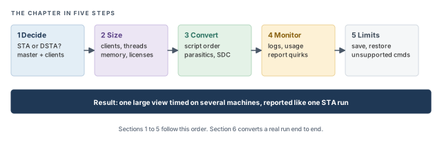
The chapter moves in five steps, from the decision to the limits of the mode. Figure 1 shows the order. Come back to it whenever you lose your place.
Key commands
Table 1 lists the commands and switches covered in this chapter, grouped by section. Each one is explained when it is first needed.
| Section | Command or switch | What it does |
|---|---|---|
| 1 Decide | tempus -distributed |
Start the tool as a DSTA master |
| 3 Convert | set_multi_cpu_usage |
Set master threads, client count and threads per client |
| 3 Convert | set_distribute_host |
Choose how and where clients are launched |
| 3 Convert | distribute_start_clients |
Launch the clients |
| 3 Convert | distribute_partition |
Split the timing graph into client slices |
| 3 Convert | update_timing -full |
Run the full timing update across all clients |
| 3 Convert | info command distribute_partition |
Tcl test that tells a DSTA session from an STA session |
| 4 Monitor | tempus -log, -overwrite |
Name the master log, or reuse an existing one |
| 4 Monitor | distribute_print_client_usage, report_resource |
Show client and resource usage |
| 5 Limits | save_design, read_design -cell |
Save and restore a DSTA session |
| 5 Limits | write_sdf, write_twf, report_disk |
Outputs and checks that work in DSTA |
1 STA versus DSTA
1.1 The concept
Let us start with ordinary STA. One process runs on one machine and uses several threads. You start it with tempus, or tempus -no_gui for a console session. As a rough guide, this copes well with designs under about 15M instances.
Above that size, two limits appear. First, one machine has only so many cores, so extra threads stop helping. Second, one machine has only so much memory. The full design, its parasitics and its timing data must all fit inside it.
DSTA removes both limits by splitting the work over several machines. It has two kinds of process:
- The master holds the full design. It splits the timing graph and collects results.
- Each client holds one slice of the timing graph and times only that slice.
You start a master with tempus -distributed. The master has no GUI. Thus, all DSTA work is done through scripts and the console.
1.2 How the work is shared
A simple way to picture a DSTA run is a team that marks a large exam. One head examiner keeps the full answer sheet. Each helper marks a stack of pages, and the head examiner collects the marks.
In the same way, a DSTA run moves through four stages:
- The master starts and launches the clients.
- The master loads the design and its parasitics.
- The master splits the timing graph into slices, one per client.
- Each client times its slice in parallel, and the master gathers the results into one set of reports.
Figure 2 shows the result of stage 3: one master and four clients, each with its own slice.
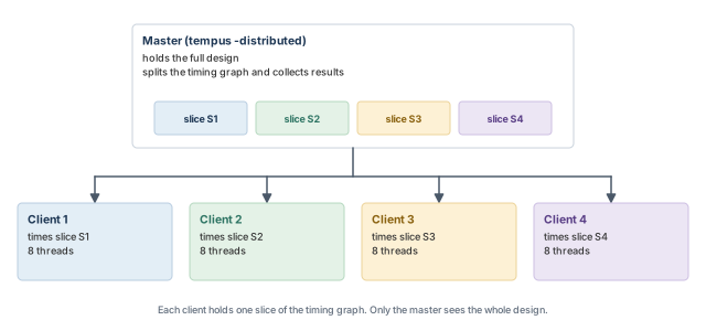
Thus, the gain comes from stage 4. If four clients each time a quarter of the graph, the timing work runs in parallel on four machines. The real speed-up is smaller than four, because the master must split, coordinate and merge.
- Exam pages are independent. Timing paths are not: a path can cross from one slice into another, and the tool must account for that.
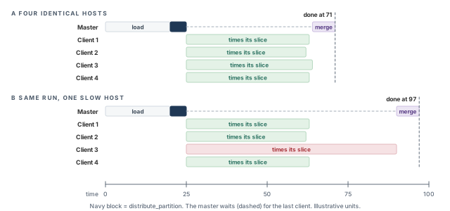
- A helper can mark at any pace. In DSTA, the master waits for every client, so the slowest client sets the pace.
Figure 3 shows where the time goes in such a run. The master loads and splits the design, then waits while the clients work. It merges only when the last client ends. Thus, in case B, one slow host delays the whole run, even though the other three clients finished early.
1.3 Why it matters
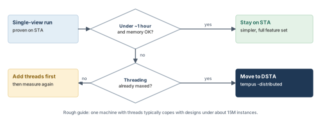
DSTA adds machines, licenses and moving parts. Thus, it is only worth using when STA has truly run out of room. Use DSTA when two things are both true:
- STA threading is already at its useful maximum.
- The runtime is still too long.
If an STA run finishes in under about one hour, and memory is fine, stay on STA. It is simpler, and every command is available.
Let us consider two cases. A 6M-instance block finishes in 40 minutes on STA. Moving it to DSTA would add licenses and script changes for little gain, so it stays on STA. A 30M-instance full-chip view takes 5 hours with threads already maxed. Here DSTA is the right move. Both runtimes are illustrative.
Figure 4 shows this decision as a flow.
1.4 Commands that exist only in DSTA
Three commands are found only in a DSTA session:
set_distribute_host– chooses how clients are launched, for example through LSF.distribute_start_clients– launches the clients.distribute_partition– splits the timing graph into slices for the clients.
Because STA does not know these commands, a script that uses them typically fails in a plain STA session. Section 3.5 shows how one script can still serve both modes.
2 Sizing a distributed run
2.1 Clients, threads and memory
Sizing means choosing the number of clients, the threads per client and the memory per machine. Getting it wrong costs either time or machines. Too few clients leaves the run slow. Too many clients waste licenses and hosts, and add coordination work for the master.
A good starting point is:
- 4 clients with 8 threads each. Measure this first, then adjust.
- About one more client per ~15M instances. Use this to grow the layout when runtime is still too long.
- Homogeneous clients. Use machines of the same type for all clients. A slow client holds back the whole run, because the master waits for every slice (Figure 3, case B).
- About 1.5 GB of memory per million instances, as a planning figure.
Let us size a 30M-instance design as an example:
- Memory: 30 × 1.5 = 45 GB, as a planning figure for the design data.
- Clients: start at 4 clients × 8 threads, which is 32 client threads.
- Measure the first run. If runtime is still too long, add clients one at a time. The ~15M rule suggests up to two more here (30M ÷ 15M = 2), but measure after each one.
Figure 5 shows this as a loop. Each pass changes one thing, then measures again.
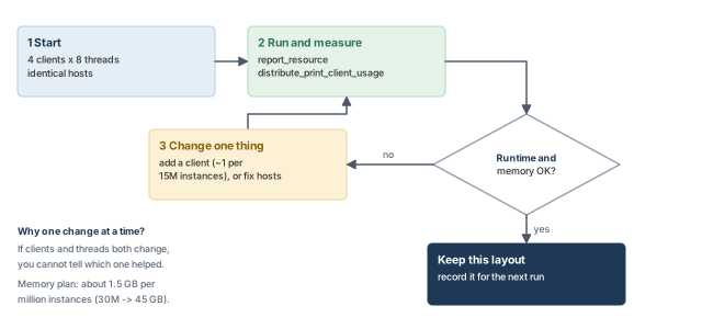
These numbers are starting points, not guarantees. Thus, always confirm memory with the resource reports after the first run, and correct the plan from real data.
Change one thing at a time when tuning. If you add clients and threads together, you cannot tell which change helped.
2.2 Inputs that speed up DSTA
Loading data is a large part of any big run. Four input choices make a distributed run faster:
- LDB libraries – compiled libraries, which typically load faster than text Liberty files.
- RCDB parasitics – a parasitic database, which typically loads faster than SPEF text.
- Tcl-predefined constraints – constraints already prepared in Tcl form, ready to read.
- Fast local disks – for the run folder and the scratch area.
The reason is simple. Every minute spent parsing text or waiting on a slow network disk is a minute in which the clients sit idle.
The scratch area rule from Getting Started with Tempus also applies here. Set TMPDIR to a large local disk before launch.
2.3 Licenses
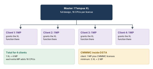
DSTA needs the Tempus XL feature set. The license count for a single-view DSTA run is:
- Master: 1 Tempus XL (16 CPUs).
- Each client: 1 MP license. The MP license grants the XL function on that client.
- Extra CPUs: each additional MP adds 16 CPUs.
Figure 6 maps these licenses onto the master and clients. For example, a run with 4 clients needs 1 XL for the master and 4 MP for the clients. For a multi-view (CMMMC) analysis inside DSTA, the master holds 1 XL. Each client holds 1 MP plus the CMMMC licenses. The minimum is 3 XL plus 2 MP. Getting Started with Tempus covers the full license tables.
A beginner launches eight clients but only four MP licenses are free. The run then typically cannot start all its clients. Count one MP per client before the run, so the shortage is found before the job is submitted.
3 Converting an STA script to DSTA
3.1 The rules
Let us convert a working STA script. Five rules govern the conversion:
- Prove the single view in STA first. Debug constraints and data on one machine, where every command and the GUI work. DSTA is a speed tool, not a debug tool.
- Use at least two clients. With one client, there is nothing to split.
- Call
set_multi_cpu_usagebefore starting the clients. The clients are launched with these settings, so later changes come too late. - Read parasitics before
distribute_partition. - Read constraints after
distribute_partition.
Rules 4 and 5 are the ones beginners break. Many STA scripts read the SDC before the SPEF, as in Design Import. In DSTA, the SPEF must come before the partition and the SDC after it. A simple way to remember it: load the design and its wires, then split. After the split, apply the constraints.
3.2 The DSTA script
The script below is a complete single-view DSTA run. Figure 7, after it, shows the same order as a flow.
set_multi_cpu_usage -cpuPerRemoteHost 4 -localCpu 4 -remoteHost 2   ;# before clients start
set_distribute_host -timeout 300 -lsf -queue lnx64 \
  -args {-n 4 -R "(CPUS>=4) span[hosts=1] rusage[mem=15000]"}   ;# launch clients via LSF
distribute_start_clients                       ;# start the clients
read_verilog top.v                             ;# netlist
read_lib slow.lib                              ;# libraries
set_top_module top                             ;# link the design
read_spef top.spef.gz                          ;# parasitics: BEFORE the partition
distribute_partition                           ;# split the graph into client slices
read_sdc top.sdc                               ;# constraints: AFTER the partition
update_timing -full                            ;# full timing on all clients
distribute_print_client_usage                  ;# check client usage
report_timing -late -max_paths 200000 -nworst 1 -path_type full_clock -net \
  > rt_max.rpt.gz                              ;# graph-based setup report
report_timing -retime path_slew_propagation -max_paths 200000 -nworst 1 \
  -path_type full_clock > rt_pba.rpt.gz        ;# path-based report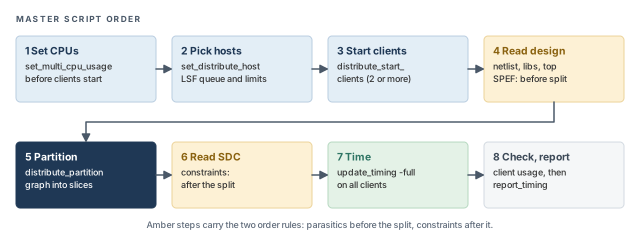
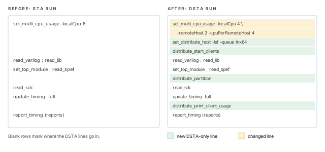
How different is this from the STA script? Figure 8 compares the two scripts side by side. Most lines stay the same. The changes are the CPU line, three new commands and one monitoring line.
read_spef stays above distribute_partition, while read_sdc stays below it.3.3 Command breakdown
Let us go through the new and changed lines one at a time.
set_multi_cpu_usage sets the thread layout of the run. It must come before distribute_start_clients.
-localCpu– the threads used by the master. The master splits, coordinates and merges, so it needs some threads of its own.-remoteHost– the number of client hosts in this layout. In the script it is 2, so two clients start. Remember the rule of at least two clients.-cpuPerRemoteHost– the threads each client uses. In the script it is 4. Thus, the clients together run 2 × 4 = 8 threads.
set_distribute_host chooses how and where the clients start.
-lsf– submits the clients to the LSF batch system, which places jobs on compute hosts.-queue lnx64– names the LSF queue to submit to. Use the queue your site reserves for large timing jobs.-args– passes extra submit options to LSF, such as the slot count and the host resource string. Section 3.4 explains the string.-timeout 300– how long the master waits for the clients. Confirm the unit withhelp set_distribute_hostbefore tuning it.
distribute_start_clients launches the clients with the settings above. If licenses or hosts are short, this is typically where the run stalls.
distribute_partition splits the timing graph into one slice per client. The parasitics must already be loaded when it runs (rule 4).
update_timing -full runs the complete timing update across the master and all clients. This is the step that takes the long runtime, and the step that DSTA speeds up.
distribute_print_client_usage prints how the clients are doing. It is non-blocking, so it does not hold up the run.
The two reports are ordinary report_timing calls. The first is a graph-based late (setup) report, with full clock paths and net rows. The second uses -retime path_slew_propagation for path-based retiming, covered in Path-Based and Robustness Analysis. Both ask for up to 200000 paths with one worst path per endpoint.
3.4 Choosing LSF hosts
On a shared compute farm, you rarely want "any free host". Some hosts are slow, some are busy, and some are reserved. The -R resource string inside -args selects hosts for the clients. Figure 9 breaks one submit string into its parts.
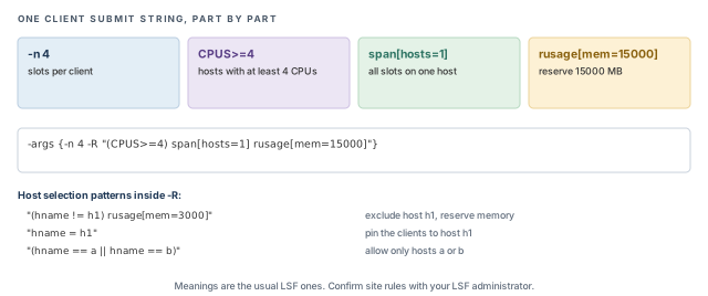
span[hosts=1] keeps all slots of one client on one machine, so its threads share memory.Three host-selection patterns are common:
-R "(hname != h1) rusage[mem=3000]" # exclude host h1, reserve memory
-R "hname = h1" # pin clients to host h1
-R "(hname == a || hname == b)" # allow only hosts a or b- Exclude a host when it is known to be slow, overloaded or unstable.
- Pin clients to one host when you must reproduce a run on the same machine.
- Group a list of hosts when only some machines have enough memory or the right type.
Exclude a host that is known to be slow or overloaded. Since the master waits for every client, one slow host sets the pace for the whole run.
3.5 One script for both STA and DSTA
It is better to keep one run.tcl for both modes. The reason is maintenance: one script means one place to fix a constraint. Two copies drift apart, and the STA and DSTA results then differ for reasons nobody can find.
The test is whether distribute_partition exists in the running session. Tcl's info command returns the command name if it exists, and an empty string if it does not. Figure 10 shows the branch.
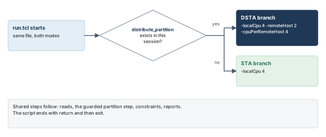
if {[info command distribute_partition] != ""} {   ;# true only in a DSTA session
  set_multi_cpu_usage -cpuPerRemoteHost 4 -localCpu 4 -remoteHost 2
} else {                                          ;# plain STA session
  set_multi_cpu_usage -localCpu 4
}
# shared reads, partition step, constraints and reports follow here
return                                            ;# end of the flow
exit                                              ;# then leave the tool
End the script with return, then exit, as shown. STA does not know the DSTA-only commands later in the script. Thus, set_distribute_host, distribute_start_clients and distribute_partition need the same guard.
Reading the SDC before distribute_partition looks harmless, since the same lines work in STA. Keep the order rule: parasitics before the partition, constraints after it.
4 Logs, monitoring and report differences
4.1 Where the logs go
A DSTA run writes one log for the master and one per client. When something goes wrong, you usually need both. The master log shows what was asked. A client log shows what failed there. Figure 11 shows a run folder after a 4-client run.
- Master log. Set its name with
tempus -log <name>. The default is./tempus.log. A new run auto-increments the name, so old logs are kept. Add-overwriteto reuse the same file. - Client logs. Each client writes
partOutput_<N>/tempus.log. The numbering can drift between runs with different client counts. Thus, check the file timestamps before trusting a client log.
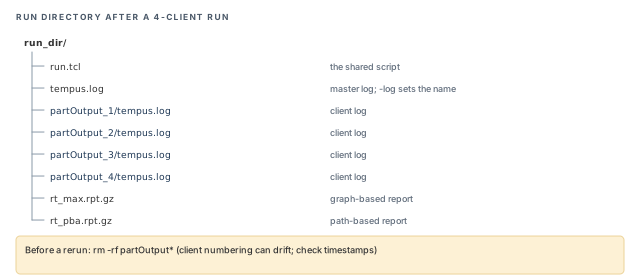
Let us see why the drift matters. Suppose yesterday's run used 6 clients and today's run uses 4. Folders partOutput_5 and partOutput_6 are still there from yesterday. If you open them, you debug a run that no longer exists. Figure 12 shows the problem and the cleanup.
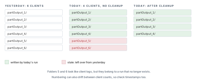
rm -rf partOutput*, only today's four folders remain.Thus, remove old client folders before a rerun:
% rm -rf partOutput*                      ;# delete old client logs and data
% tempus -distributed -log blkA_dsta.log  ;# start a fresh master with a named log
4.2 Monitoring a running job
A long distributed run should not be a black box. Two commands show how the run is using its resources:
report_resource– reports how the session is using resources, such as memory and runtime.distribute_print_client_usage– shows client usage. It is non-blocking, so it does not hold up the run.
Use them right after update_timing -full. Their numbers tell you whether the memory plan was right, and whether one client was much busier or slower than the rest.
4.3 How reports differ
DSTA reports are expected to carry the same timing, but three habits change:
- Order. Without sort criteria, the report order is arbitrary. Add sort criteria when order matters, for example when comparing with an STA report.
- No path numbers. DSTA reports do not number the paths. Do not write scripts that parse path numbers.
- No
-tcl_list. The-tcl_listoption onreport_*commands is not supported.
These differences matter most to post-processing scripts. A script that reads "path 1" or relies on line order breaks silently, even when every slack is identical. Figure 13 shows a small example.
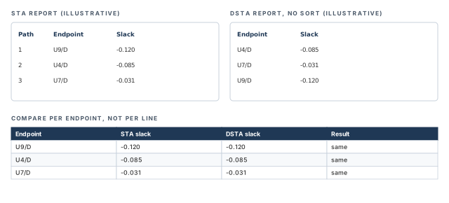
When you compare DSTA against the earlier STA run, compare slack values per endpoint, not line by line. Line order and path numbers may differ, even when the timing is identical.
partOutput* before reruns, and never rely on report order or path numbers.5 What works in DSTA and what does not
5.1 Supported outputs and session files
Several outputs work normally in DSTA:
write_sdf– writes the delay file for simulation.write_twf– writes the timing window file, which other runs can read for crosstalk analysis.report_disk [-dir d]– reports disk use, optionally for one folder. This helps, because DSTA runs write a lot of data.
5.2 Saving and restoring a session
Saving lets you reload a timed design without repeating the long load and update. In DSTA it works with limits. Figure 14 shows the key rule.
save_design <session> [-overwrite]saves the session. The saved data is about 2× the size of a flat save. The-cellviewand-noRCoptions are not available.read_design <dir> -cell <cell>restores it. The number of clients must match the save. The thread count may change. The-cellviewand-physical_dataoptions are not available.
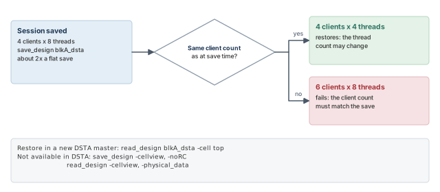
A simple way to picture the rule: the saved data is stored per slice. Four slices need four clients to load them, but each client may use more or fewer threads.
save_design blkA_dsta -overwrite        ;# about 2x the size of a flat save
# later, in a new DSTA master started with the same client count:
read_design blkA_dsta -cell top ;# restore; threads per client may differPlan disk space before saving. If a flat save of the block takes 40 GB, budget about 80 GB for the DSTA save. Both numbers are illustrative.
5.3 Commands that are not supported
Many commands do not work in DSTA. Table 2 groups them by family. If your STA script uses one of them, keep that step in a separate STA run.
| Family | Commands |
|---|---|
| GUI and preferences | the GUI, get_preference, set_preference |
| Design data and session | read_def, write_def, write_rcdb, free_design, check_multi_cpu_usage |
| Distributed MMMC | distribute_command, distribute_views, distribute_read_design, set_distribute_variables, get_distribute_variables |
| Reports and analysis | read_boundary_model, merge_timing_reports, report_clock_sense, report_design_rule, report_cell_instance_timing, report_pba_aocv_derate, set_exclude_net, write_loop_break_sdc |
| Noise | report_voltage_swing, write_noise_eco |
| Timing models | do_extract_model, write_model_timing, merge_model_timing, compare_model_timing, all ILM and PTM commands |
| Path analysis and netlist edits | analyze_paths_by_*, delete_net, detach_module_port |
| ECO and placement | eco_opt_design, get_eco_opt_mode, read_partition, set_place_mode, set_filler_mode |
| Power | report_power, set_power*, write_tcf |
| Extraction and others | extract_rc, rc_out, report_rcdb, CTD window commands, set_msv_mode |
Two related limits appear in other chapters:
- In DRV reporting,
-worst_drv_per_netand the fieldstransition_si,max_slackandmin_slackare not supported in DSTA. See Advanced Checks and Timing Debug. write_timing_context -with_constraintscannot run from DSTA. See Hierarchical Timing Context.
5.4 Planning a flow around the limits
The list looks long, but the pattern is simple. DSTA is for timing a very large view and reporting it. Work that changes the design, builds models, analyzes power or uses the GUI happens elsewhere.
Thus, a typical full-chip flow has three kinds of session:
- A DSTA session that times the full view and writes reports, SDF and timing windows.
- Separate sessions for signoff fixing, covered in Signoff ECO.
- Separate sessions for model extraction, covered in Timing Models.
Figure 15 shows this split for one full-chip view.
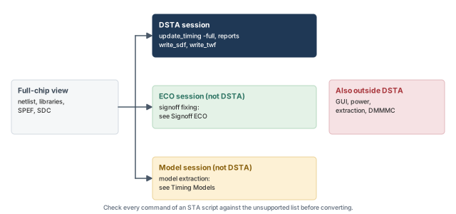
Check every command in an STA script against Table 2 before converting it. One unsupported command found early saves a failed overnight run.
6 Worked example: moving a large block to DSTA
Let us convert one real run. The assumptions are written as comments at the point of use.
The task. A 30M-instance block has one setup view. On STA with threads maxed, update_timing -full takes about 5 hours. That is too long for nightly runs. The STA script is already clean.
Step 1 – decide
The run is over one hour and threading is maxed. From Figure 4, the run moves to DSTA. We also check the script against Table 2. It uses no unsupported commands, so no step needs to move to a separate session.
Step 2 – size and license
We start at the recommended 4 clients × 8 threads on identical hosts. The memory plan is 30 × 1.5 = 45 GB (illustrative). Licenses: 1 XL for the master and 4 MP, one per client. We clean old client folders first, so the logs we read later belong to this run.
# Assuming TMPDIR is already set to a large local disk
% rm -rf partOutput*                                ;# clean old client data
% tempus -distributed -log blkA_dsta.log            ;# master with a named log
Step 3 – the converted script
Host h7 is known to be slow, so we exclude it. The -n 8 slot count matches the 8 threads per client.
# Assuming LSF queue lnx64 and slow host h7 to avoid
set_multi_cpu_usage -localCpu 8 -remoteHost 4 -cpuPerRemoteHost 8   ;# 4 clients x 8
set_distribute_host -timeout 300 -lsf -queue lnx64 \
  -args {-n 8 -R "(hname != h7) rusage[mem=15000]"}      ;# skip host h7
distribute_start_clients                                 ;# launch 4 clients
read_verilog blkA.v.gz                                   ;# netlist
read_lib slow.lib                                        ;# libraries
set_top_module blkA                                      ;# link
read_spef blkA.spef.gz                                   ;# parasitics before split
distribute_partition                                     ;# split the graph
read_sdc blkA.sdc                                        ;# constraints after split
update_timing -full                                      ;# full update
distribute_print_client_usage                            ;# check the clients
report_resource                                          ;# memory and runtime
report_timing -late -max_paths 200000 -nworst 1 -path_type full_clock -net \
  > rt_max.rpt.gz                                        ;# setup report
save_design blkA_dsta                                    ;# about 2x a flat save
return                                                   ;# end of the flow
exit                                                     ;# leave the tool
Notice the two order rules in the middle of the script. read_spef sits above distribute_partition, and read_sdc sits below it.
Step 4 – check the result
- Compare endpoint slacks with the last STA run. They are expected to match, even though the order differs. Investigate any endpoint that does not.
- Check each
partOutput_<N>/tempus.logtimestamp, so you read this run's logs. - Look at
distribute_print_client_usage. If one client is much slower, exclude its host next time (Figure 3, case B). - Use the memory figures from
report_resourceto correct the 45 GB plan for the next run. - Note that the session was saved with 4 clients. Any restore must also use 4 clients.
The 5-hour runtime and 45 GB memory figures are illustrative. Your own numbers come from report_resource on the first run.
7 Common mistakes and how to catch them
Table 3 gathers the mistakes from this chapter. Each row gives the symptom you would see first.
| Symptom | Likely cause | Fix |
|---|---|---|
| Constraints missing or slack differs from STA | Constraints read before distribute_partition |
Read SPEF before the partition and SDC after it |
| Clients start with the wrong thread count | set_multi_cpu_usage placed after distribute_start_clients |
Set CPUs before starting clients |
| Run stalls at client launch | Not enough MP licenses, or no free LSF hosts | Count one MP per client; check the LSF queue |
| One client is much slower than the rest | Mixed machine types | Use homogeneous hosts; exclude slow ones with -R |
| Debugging the wrong client log | Old partOutput* folders, drifted numbering |
rm -rf partOutput* before reruns; check timestamps |
| Script parsing path numbers breaks | DSTA reports have no path numbers | Parse endpoints and slack instead |
| Report diff shows huge changes | Report order is arbitrary without sort criteria | Sort, or compare per endpoint |
read_design fails on restore |
Different client count than at save | Restore with the same number of clients |
| A command errors out only in DSTA | Command not supported in DSTA | Move that step to a separate STA run |
Script fails in STA on distribute_partition |
DSTA-only command with no mode test | Guard it with info command distribute_partition |
| DSTA is slower than expected | Text libraries and SPEF, slow network disks | Use LDB, RCDB, Tcl-predefined constraints, local disks |
8 Interview preparation
STA runs one multi-threaded process on one machine. DSTA uses a master with the full design, plus clients that time graph slices.
- DSTA starts with
tempus -distributedand has no GUI. - The master splits the graph and merges the results.
- The clients each time one slice in parallel.
When STA finishes in under about an hour and memory is fine.
- DSTA adds licenses, hosts and script rules.
- It is for runs where threading is maxed and runtime is still too long.
read_spef and read_sdc go relative to distribute_partition?Parasitics before the partition, constraints after it.
- Many STA scripts read the SDC first, so beginners carry that habit over.
- Getting it wrong is the most common conversion error.
set_multi_cpu_usage come before distribute_start_clients?The clients are launched with those CPU settings, so they must be set first.
-remoteHostsets the client count and-cpuPerRemoteHostthe threads per client.-localCpusets the master's own threads.
Start with 4 clients of 8 threads on identical machines, and plan about 1.5 GB per million instances.
- Add roughly one client per ~15M instances if runtime is still too long.
- Correct the plan from
report_resourceafter the first run.
The master waits for every client, so the slowest machine sets the pace.
- One slow host can erase the gain from the others.
- Exclude slow hosts with an LSF
-Rstring.
One Tempus XL for the master and one MP per client, so four MP.
- The MP license grants the XL function on each client.
- Each extra MP adds 16 CPUs.
Test [info command distribute_partition] and pick the CPU layout from the result.
- The command exists only in a DSTA session.
- One script keeps constraint fixes in one place.
In partOutput_<N>/tempus.log, one folder per client.
- Numbering can drift between runs with different client counts.
- Check timestamps and clean
partOutput*before a rerun.
DSTA reports have no path numbers, and the order is arbitrary without sort criteria.
-tcl_listonreport_*is also unsupported.- Parse endpoints and slack instead.
No. The client count must match the save; only the thread count may change.
save_designoutput is about 2× a flat save.-cellview,-noRCand-physical_dataare not available.
eco_opt_design or do_extract_model in a DSTA session?No. ECO, model extraction, power and distributed MMMC commands are not supported in DSTA.
- Run those steps in their own sessions.
- Check a script against the unsupported list before converting it.
Chapter recap
Key takeaways
- DSTA uses one master with the full design and clients that each time a slice of the graph.
- Move to DSTA only when STA threading is maxed and the run is still too long.
- Start with 4 clients × 8 threads on identical hosts; plan about 1.5 GB per million instances.
- Set CPUs before clients start. Read SPEF before
distribute_partitionand SDC after it. - Keep one script for both modes, guarded by
info command distribute_partition. - Name the master log, clean
partOutput*, and check client log timestamps. - Do not rely on report order, path numbers or
-tcl_listin DSTA. - Restore a saved session with the same client count. ECO, models, power and GUI are not available.
Command recap
| Command or switch | Purpose |
|---|---|
tempus -distributed |
Start a DSTA master (no GUI) |
set_multi_cpu_usage -localCpu -remoteHost -cpuPerRemoteHost |
Master threads, client count, threads per client |
set_distribute_host -lsf -queue -args -timeout |
How and where clients start |
distribute_start_clients |
Launch the clients |
distribute_partition |
Split the timing graph |
update_timing -full |
Full timing update |
distribute_print_client_usage, report_resource |
Monitor clients and resources |
tempus -log, -overwrite |
Name or reuse the master log |
save_design -overwrite, read_design -cell |
Save and restore a DSTA session |
write_sdf, write_twf, report_disk -dir |
Supported outputs and checks |
Compact glossary
| Term | Meaning |
|---|---|
| DSTA | Distributed STA: one analysis split across several machines |
| Master | The process that holds the full design and collects results |
| Client | A process on another machine that times one graph slice |
| Partition | Splitting the timing graph into client slices |
| Homogeneous clients | Clients on machines of the same type and speed |
| LSF | A batch system that places jobs on compute hosts |
| Resource string | The -R text that tells LSF which hosts and resources to use |
| LDB | A compiled library format that typically loads faster than Liberty text |
| RCDB | A parasitic database that typically loads faster than SPEF text |
| partOutput folder | The per-client output and log folder |
Practical perspective
On a real project, DSTA usually arrives late, when full-chip views grow beyond one machine. Teams that keep one shared run.tcl for STA and DSTA convert quickly. Teams that fork the script often spend a long time chasing small differences. Thus, prove the view in STA, keep one script, and let the mode test pick the CPU layout.
What comes next
The design is now timed, even at full-chip size. The next step is to fix what fails. In Signoff ECO, we use the tool to repair setup, hold, DRV, SI, IR and EM problems. The fixes are then written back for implementation.