Chapter overview
Every slack number in a timing report is a sum of delays. If one delay is wrong, every path through it is wrong. Thus, before we trust any report, we need to know how the tool calculates a single delay.
Base delay is the delay of a cell or a wire with no crosstalk effects. The tool computes it from three things: the library tables, the input waveform and the load on the output. Crosstalk is added on top of it later, in Signal Integrity Delay Analysis.
Why spend a whole chapter on one number? Because most strange timing results end here. Think of a path that fails by 10 ps, or a result that changes between two runs. The cause is often one delay, calculated from poor data or with the wrong setting.
This chapter starts from the basic building blocks: cell delay, net delay, slew and load. Then we look at how libraries describe a cell and run the base delay flow. Next, we control how waveform shapes travel from stage to stage, and check that the libraries support it. We finish with reading delay reports and the limits of what any calculation can deliver.
Learning objectives
- Explain the difference between a cell delay and a net delay, and how input slew and output load affect each.
- Describe how a lookup table gives a delay, and why CCS and ECSM libraries are preferred.
- Run the base delay flow in the right order, starting with
set_design_mode -process. - Use
report_timingandreport_delay_calculationto inspect one timing arc. - Choose between the
no_propagationandpropagationsettings of the equivalent waveform model, and state their costs. - Check a library against the requirements for waveform propagation, including the rules at 16nm and below.
- Read a
report_timing -netreport and change its columns withreport_timing_format. - Explain why a negative cell delay is not an error, and why SDF-annotated arcs skip delay calculation.
Chapter roadmap
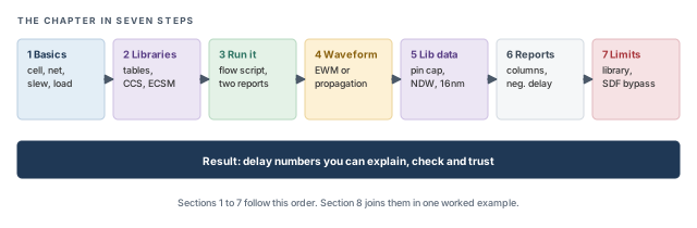
The chapter moves in seven steps, from the parts of one delay to the limits of the result. Figure 1 shows the order. Come back to it whenever you lose your place.
Key commands
Table 1 lists the commands and settings in this chapter, grouped by section. Each one is explained when it is first needed.
| Section | Command or setting | What it does |
|---|---|---|
| 3 Running the flow | set_design_mode -process |
Sets the process node, which chooses node-based defaults |
| 3 Running the flow | read_lib, read_verilog, set_top_module, read_sdc, read_spef |
Load libraries, netlist, top module, constraints and parasitics |
| 3 Running the flow | report_timing |
Reports timing paths with their delays and slack |
| 3 Running the flow | report_delay_calculation -from -to |
Shows how the delay of one arc was calculated |
| 4 Waveforms | set_delay_cal_mode -equivalent_waveform_model |
Chooses no_propagation or propagation of waveform shapes |
| 5 Library data | normalized_driver_waveform (Liberty attribute) |
Describes the driver waveform; use the active form, not the analytical one |
| 6 Reports | report_timing -net |
Lists net arcs and cell arcs in the path report |
| 6 Reports | set_global report_timing_format |
Chooses the columns of the timing report |
| 7 Limits | read_sdf |
Annotates delays from a file; those arcs skip delay calculation |
1 The building blocks of a delay
1.1 One stage of logic
A timing path is a chain of small pieces. Each piece is called a stage. Once we understand one stage, a whole path is just the same idea repeated.
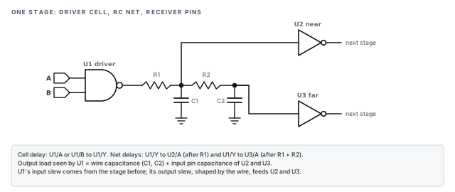
Let us consider the stage in Figure 2. It has three parts:
- The driver cell – here the NAND gate
U1. It switches its output when an input changes. - The net – the wire from
U1/Yto its receivers. It has resistance (R) and capacitance (C), drawn here as two R–C sections. - The receivers – the input pins of
U2andU3. They are the next stage's inputs.
1.2 Cell delay and net delay
The cell delay is the time from a driver's input pin to its output pin, for example U1/A to U1/Y. It is the time the transistors inside the cell need to switch and charge the output.
The net delay is the time from the driver's output pin to one receiver's input pin, for example U1/Y to U3/A. It is the time the edge needs to travel along the resistive wire.
Each receiver has its own net delay. In Figure 2, U2 sits closer to the driver than U3. Thus, the edge reaches U2/A first, and U3/A later. The tool reports a separate net arc for each receiver.
1.3 Slew and load
Two numbers control a cell delay:
- Input slew – how fast the input signal changes. A slow input edge turns the transistors on gradually, so the cell responds later.
- Output load – the capacitance the cell must charge or discharge. A larger load needs more charge, so the output also moves more slowly.
The load seen by U1 is the wire capacitance (C1 and C2) plus the input pin capacitance of U2 and U3. Thus, adding a receiver, or lengthening the wire, makes the driver slower.
Figure 3 shows how delay and slew are measured on real waveforms. Delay is taken from the 50% point of the input to the 50% point of the output. Slew is the time between two voltage thresholds on one edge, for example 20% and 80%.
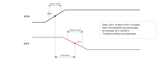
- The exact thresholds are defined in the library, not by the designer. Different libraries can use different thresholds.
- All times in this chapter are in ns and all capacitances in pF, unless said otherwise.
Figure 4 shows both effects on one inverting cell, with illustrative numbers. A rising edge on A gives a falling edge on Y. Each panel changes one input and keeps the other fixed.
- Panel A – heavier load. The input slew stays at 0.02 ns. The load grows from 0.01 pF to 0.10 pF. The delay grows from 0.040 ns to 0.120 ns, and the output edge becomes much slower.
- Panel B – slower input. The load stays at 0.01 pF. The input slew grows from 0.02 ns to 0.30 ns. The delay grows from 0.040 ns to 0.081 ns.
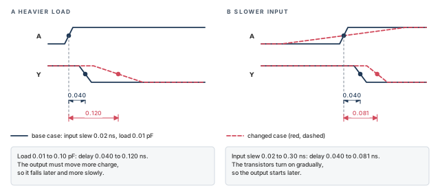
Thus, the two inputs are not equal partners. In this example, ten times more load triples the delay. Fifteen times more input slew only doubles it. Real cells differ, but both effects are always present.
1.4 How slews travel along a path
The output slew of one stage is the input slew of the next. However, the wire changes the edge on the way. Figure 5 shows the same edge at three pins of the stage in Figure 2.
Let us follow the edge with illustrative numbers. Assume U1/Y crosses 50% at 0.300 ns with a slew of 0.040 ns. The near pin U2/A crosses 50% at 0.304 ns, so its net delay is 0.004 ns. The far pin U3/A crosses at 0.312 ns, so its net delay is 0.012 ns. Its slew has also grown, for example to 0.060 ns.
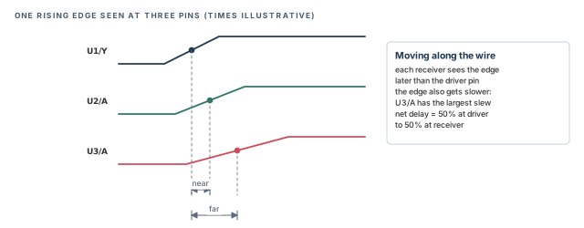
Thus, a long wire hurts twice. It adds net delay, and it slows the edge, which makes the next cell slower too.
2 How libraries describe a cell
2.1 Lookup tables
The tool does not simulate transistors during timing analysis. It would be far too slow for millions of cells. Instead, it reads delays from tables that the library team built once, by simulation, for every cell.
The simplest library model stores delays in a two-dimensional table. One axis is input slew and the other is output load. Each entry is the delay measured for that pair. A similar table gives the output slew.
Let us consider panel A of Figure 6. The tool needs the delay for a slew of 0.10 ns and a load of 0.075 pF. That point is not in the table. It lies halfway between the entries 0.092 ns (at 0.05 pF) and 0.138 ns (at 0.10 pF). Thus, the tool interpolates:
- Halfway in load means halfway in delay.
- 0.092 + 0.5 × (0.138 − 0.092) = 0.115 ns.
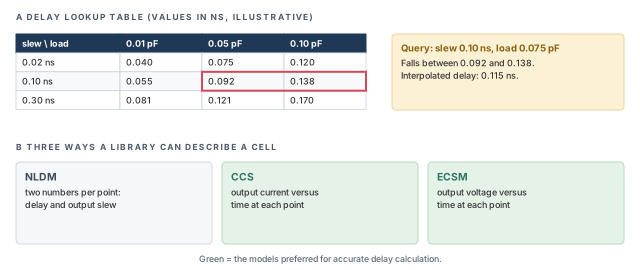
This model is called NLDM (nonlinear delay model). It is fast and simple. However, it stores only two numbers per point: a delay and an output slew.
2.2 Why CCS and ECSM are preferred
A single slew number assumes the output edge is a straight ramp. Real edges are curved, and the curve shape changes how the next stage switches. At small nodes, the error from that assumption can become large enough to matter.
Modern libraries therefore store more detail at each table point:
- CCS (composite current source) stores the output current over time. The tool can rebuild the voltage waveform for any load from that current.
- ECSM (effective current source model) stores the output voltage over time, at several thresholds.
Both let the tool rebuild the real waveform shape instead of guessing it from one number. For this reason, CCS and ECSM libraries are preferred for delay calculation.
On a new project, ask early which model your libraries use. If only NLDM is available at an advanced node, expect more pessimism and plan more margin. The settings later in this chapter need CCS or ECSM data to help.
2.3 Noise data for later chapters
Crosstalk analysis needs extra noise library data on top of the timing data. Roughly, it describes how a cell resists being disturbed by a neighboring wire. The supported forms are CCS-N, ECSM-SI and cdB.
Base delay does not use this data. However, it is worth checking now that the noise data exists, because Signal Integrity Delay Analysis depends on it.
3 Running base delay calculation
3.1 The flow
Figure 7 shows the base delay flow. It has five steps, and the order matters. Note that the process node is set before anything is read.
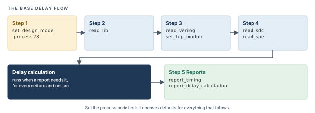
The steps are:
- Set the process node with
set_design_mode -process. - Read the libraries with
read_lib. - Read and link the netlist with
read_verilogandset_top_module. - Read the constraints and parasitics with
read_sdcandread_spef. - Report with
report_timingandreport_delay_calculation. Delay calculation typically runs when a report first needs it.
3.2 Why the process node comes first
The command set_design_mode -process tells the tool the technology node, in nm. For example, -process 28 means a 28nm design. The tool uses it to choose default settings that suit that node.
Think of it as telling a new colleague which project they are on before handing over the files. The defaults are chosen once, at the start. It is better to make this the first command of every script. If it comes later, the data already read might not get the intended defaults. Two scripts with the same data could then give different delays.
3.3 Command breakdown
The complete flow for a 28nm design looks like this. Assume the design is called dma_mac.
set_design_mode -process 28          ;# first: node-based defaults for 28nm
read_lib slow.lib                    ;# timing libraries (CCS or ECSM preferred)
read_verilog dma_mac.v               ;# gate-level netlist
set_top_module dma_mac               ;# link the design under its top module
read_sdc constraints.sdc             ;# clocks and constraints
read_spef cell.spef.gz               ;# wire parasitics from extraction
report_timing                        ;# worst path with delays and slack
report_delay_calculation -from inst1/A -to inst1/Y   ;# how one arc was computed
Each line has a clear job:
set_design_mode -process 28– selects 28nm defaults. Without it, the tool cannot choose node-based defaults for your design.read_lib– loads the timing libraries. Every cell in the netlist must find its model here.read_verilogandset_top_module– load the netlist and link it under the named top module.read_sdc– loads clocks and constraints. Without clocks, there are no timed paths to report.read_spef– loads the wire R and C. Without it, net delays and loads would miss the wire.
The last two commands answer different questions:
report_timingshows the whole path. It answers "is this path fast enough?"report_delay_calculation -from inst1/A -to inst1/Yshows one arc. It answers "why is this one delay this large?" Here the arc runs from inputAto outputYof instanceinst1.
3.4 Reading a delay calculation report
A delay calculation report lists the inputs the tool used for one arc. A shortened, illustrative form looks like this:
From pin     : inst1/A        To pin     : inst1/Y
Input slew   : 0.058          Load (pF)  : 0.012
Cell delay   : 0.048          Output slew: 0.071
Read it in this order:
- Input slew – is the incoming edge reasonable? A very slow slew points to a weak driver or a long wire in the stage before.
- Load – is the capacitance reasonable for the fanout? A high load points to a long wire or too many receivers.
- Cell delay and output slew – only now judge the result. They follow from the two inputs above.
When one delay in a path looks wrong, do not guess. Run report_delay_calculation on that arc first. It shows the slew and load the tool actually used, which is usually where the answer is.
report_timing for paths and report_delay_calculation for single arcs.4 Handling the waveform shape
4.1 The concept
Panel A of Figure 8 shows a real output waveform next to a simple ramp. Both cross 50% at nearly the same time. However, the real waveform has a long, slow tail near the top.
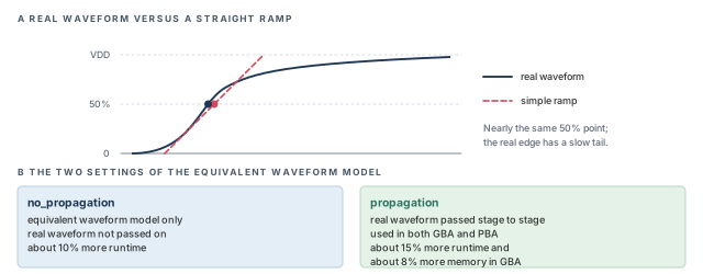
Why does the tail matter if the 50% point is the same? Because the next cell does not switch exactly at 50% of its input. It responds to the whole edge. A receiver driven by the slow tail switches later than a ramp would predict.
At large nodes this error is small, so a ramp is good enough. At small nodes, the wires are more resistive and the tails are longer. The error can then be large enough to change slack.
The tool handles this with the equivalent waveform model (EWM). It describes a real waveform shape more accurately than a single slew number does.
4.2 Command breakdown
The setting is made with set_delay_cal_mode -equivalent_waveform_model. It takes one of two values:
set_delay_cal_mode -equivalent_waveform_model no_propagation   ;# EWM only
# OR
set_delay_cal_mode -equivalent_waveform_model propagation ;# pass real waveforms onno_propagation– the tool uses the equivalent waveform model only. The real waveform is not propagated to the next stage. This costs about 10% more runtime. Use it when you want better accuracy than a plain ramp at a modest cost.propagation– the real waveform is propagated from stage to stage. Each stage receives the shape the previous stage really produced. It works in both GBA and PBA, the two analysis styles explained just below. It costs about 15% more runtime, and about 8% more memory in GBA.
4.3 GBA and PBA in brief
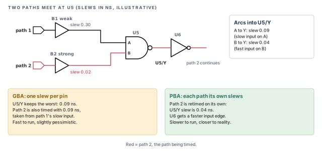
Two terms appear here. In graph-based analysis (GBA), each pin keeps one worst-case slew and arrival, shared by all paths through it. It is fast, but slightly pessimistic. In path-based analysis (PBA), the tool retimes one path at a time with that path's own slews. It is slower, but closer to reality. PBA is covered in Path-Based and Robustness Analysis.
Figure 9 shows why this matters for slews. Two paths meet at the NAND gate U5. Path 1 arrives on pin A through a weak buffer, with a slow 0.30 ns edge. Path 2 arrives on pin B through a strong buffer, with a fast 0.02 ns edge.
In GBA, the output pin U5/Y keeps only the worst slew, 0.09 ns from the A arc. Path 2 is then timed with that slow edge, even though its own edge at U5/Y is 0.04 ns. In PBA, path 2 is retimed with its own edges, so U6 sees the faster slew. Waveform propagation works in both modes, but the edge it carries in GBA is the shared worst one.
4.4 Which one to choose
Thus, propagation is the more accurate choice, and it costs more. It is better to decide based on the node and the margin you have:
- Small nodes, tight signoff – the extra runtime is usually worth it, because a few picoseconds decide the result.
- Early, fast runs –
no_propagationmight be enough, because the design will still change a lot. - Correlation work – keep the setting identical between the runs you compare, or the differences mean nothing.
A common mistake is to turn on propagation with libraries that lack the needed waveform data. The tool then has little real shape to pass on, and you pay the runtime for no gain. Check the library first, as the next section explains.
propagation carries them forward for the best accuracy, at about 15% more runtime and 8% more memory in GBA.5 Library requirements for waveform propagation
5.1 Why the library matters here
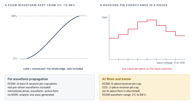
Waveform propagation can only be as good as the waveform data in the library. If a library stores too few points, the tool must fill the gaps with estimates. The result then looks precise but is not. Figure 10 shows what a suitable library contains.
5.2 Receiver pin capacitance
A receiver's input capacitance is not one fixed number. It changes while the input voltage moves, because the transistors inside change state. Panel B of Figure 10 shows this as a step curve.
A library can describe this with several values across the transition, called pieces or points. More points describe the change more faithfully. For ECSM, propagation needs at least 8 receiver pin-capacitance (pin-cap) points.
5.3 Driver waveforms and NDW
The tool also needs to know the shape of the edge that drove each cell when the library was characterized.
Figure 11 shows how a cell is typically characterized. A pre-driver cell drives the input of the cell under test, and a load sits on its output. The library team sweeps the slew and the load, and records the results in the tables.
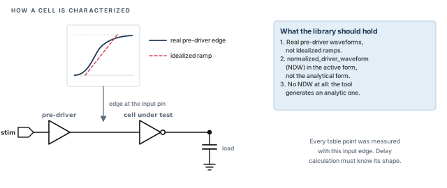
Every table entry was measured with that particular input edge. When the tool later uses the table, it must know the shape of that edge. Otherwise it compares a real edge in your design with an unknown edge in the library. Two library items describe that edge:
- Pre-driver waveforms – the library should include real pre-driver waveforms, not idealized ones. These are the input edges used when the cell was measured.
- Normalized driver waveform – the Liberty attribute
normalized_driver_waveform(NDW) stores that driver shape. It should be the active form, not the analytical form.
If a library has no NDW at all, the tool generates an analytic one automatically. The run still works. However, it is less accurate than real data, so it is better to ask the library team for NDW.
5.4 Extra rules at 16nm and below
At 16nm and below, three more rules apply:
- ECSM libraries use an 8-piece receiver pin-capacitance model.
- CCS libraries use a 2-piece receiver pin-capacitance model. An N-piece form is also listed for CCS.
- ECSM waveforms cover the range from 2% to 98% of the voltage swing, as panel A of Figure 10 shows.
The 2%–98% range matters because the slow tail lives near the top and bottom of the edge. A waveform stored only from 10% to 90% would cut the tail off.
Before enabling propagation on a new library set, ask the library team to confirm each item in Figure 10. A library that fails them still runs. However, the results are no more accurate than without propagation.
6 Reading delay reports
6.1 Seeing net delays
A path report is easiest to debug when cell delays and net delays appear on separate rows. The -net option makes report_timing list the net arcs together with the cell arcs:
tempus> report_timing -net ;# show net arcs and cell arcsWith net rows visible, you can tell at once whether a slow stage is caused by the cell or by its wire.
6.2 Choosing the columns
The global setting report_timing_format chooses which columns appear, and in which order. A useful set for delay work is:
tempus> set_global report_timing_format {hpin cell slew delay arrival} ;# report columnsEach column has one job:
hpin– the hierarchical pin name, so you can find the pin in the design.cell– the library cell at that pin.slew– the transition time at the pin.delay– the delay of the arc that ends at that pin.arrival– the running total from the path start.
6.3 Reading the report row by row
  hpin        cell      slew   delay  arrival
  inst0/CK    DFFX1    0.040  0.000   0.500
  inst0/Q     DFFX1    0.055  0.120   0.620
  inst1/A     NAND2X1  0.058  0.004   0.624
  inst1/Y     NAND2X1  0.071  0.048   0.672
  inst2/A     INVX2    0.074  0.006   0.678
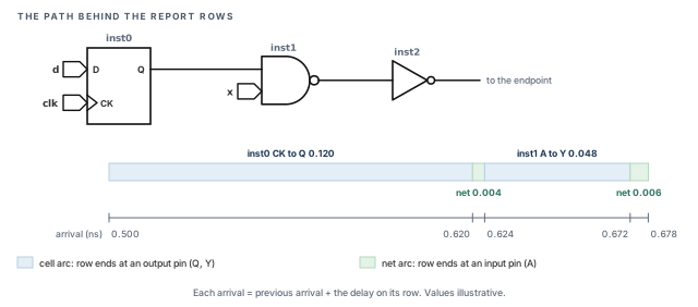
Figure 12 draws the same rows as a path and a time line. Each colored bar is one row of the report. The long bars are cell arcs and the thin bars are net arcs.
Let us read it:
- Rows ending at an input pin (
inst1/A,inst2/A) are net arcs. Their delays are small: 0.004 and 0.006 ns. - Rows ending at an output pin (
inst0/Q,inst1/Y) are cell arcs. They carry most of the delay. - Each arrival is the previous arrival plus the delay on that row. For example, 0.620 + 0.004 = 0.624 ns.
- The slew grows slightly across each net, from 0.055 to 0.058 ns and from 0.071 to 0.074 ns. That is the wire effect from Figure 5.
6.4 Negative cell delay
Sometimes a report shows a cell delay below zero. Beginners often think the tool is broken. It is not. Figure 13 shows how this happens.
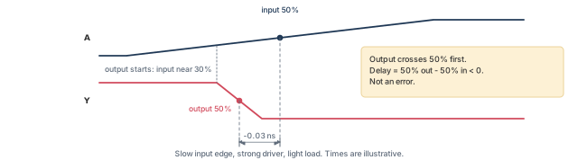
Recall that delay is measured from the 50% point of the input to the 50% point of the output. The two edges can have very different speeds. Let us consider a cell whose input edge moves slowly, while its output switches fast because it drives a light load.
The cell starts to switch as soon as its input passes its own switching level, which can be below 50%. A fast output can then complete half its swing before the slow input reaches 50%. The output crosses 50% first, and the measured difference is negative.
Note that the cell never switches before its input starts moving. Only the 50%-to-50% measurement is negative. The tool treats this as a normal result, not as an error. The path arrival still adds up correctly. The input arrival was itself measured at the late 50% point of the slow edge.
A common mistake is to treat a negative cell delay as a library or tool bug, and spend a day chasing it. Check the input and output slews first. A large mismatch between the two edges is the usual reason.
report_timing -net with hpin cell slew delay arrival to see every arc. A negative cell delay is a measurement effect, not an error.7 What limits the accuracy
7.1 The library sets the ceiling
Delay calculation reads its numbers from the library tables. Thus, the result can never be more accurate than the library content. No tool setting can recover information the library does not hold.
A coarse table, a missing waveform or a wrong pin capacitance flows straight into every path that uses that cell. For example, if one buffer's pin capacitance is 10% too low, every stage driving that buffer looks faster than it is.
It is better to review the library before tuning tool settings. Settings can only use the data that exists.
7.2 SDF annotation bypasses delay calculation
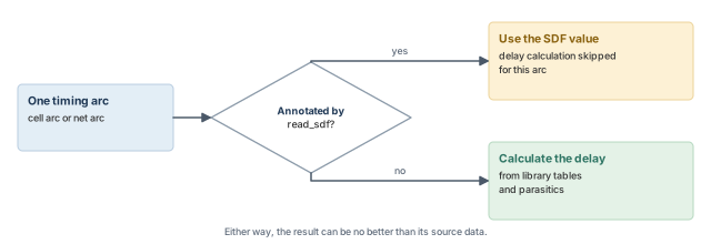
The command read_sdf annotates delays from an SDF (standard delay format) file. An SDF file holds fixed delay values per arc, usually written by another tool or an earlier run. Figure 14 shows what the tool does with each arc.
For every arc annotated by read_sdf, the tool uses the SDF value directly. No delay calculation is done for that arc. This is useful for correlation, when you want to time the design with another tool's delays.
However, it also means the annotated arcs ignore the library, the parasitics and every delay setting in this chapter. Thus, a run that mixes annotated and calculated arcs needs care.
A common mistake is to read an old SDF file into a run, then change the parasitics. The annotated arcs keep their old values. The report mixes fresh and stale delays without warning.
8 Worked example: checking one suspicious arc
The task. The 28nm block dma_mac fails setup by a small margin. One NAND gate, inst1, has a larger delay than expected. We want to know why, and whether waveform propagation changes it.
The method has four steps, and each one narrows the question:
- Load the design correctly, so the numbers can be trusted.
- See the arc inside its path, to find which delay is unusual.
- Open the arc, to see the slew and load behind that delay.
- Test the waveform setting, to see whether the edge shape matters.
Step 1 – load the design with the node set first
set_design_mode -process 28          ;# node defaults before any read
read_lib slow.lib                    ;# assuming an ECSM library
read_verilog dma_mac.v               ;# netlist
set_top_module dma_mac               ;# link
read_sdc constraints.sdc             ;# constraints
read_spef cell.spef.gz               ;# parasitics
Why this order? The node defaults must be in place before any data is read. Otherwise the result of the investigation could depend on script order rather than on the design.
Step 2 – see the arc in its path
tempus> set_global report_timing_format {hpin cell slew delay arrival}   ;# delay columns
tempus> report_timing -net                                                ;# cell and net arcs
Assume the report shows inst1/Y with a delay of 0.048 ns and an input slew of 0.058 ns at inst1/A. The net arc into inst1/A is only 0.004 ns. Thus, the wire before inst1 is not the problem. We focus on the cell arc.
Step 3 – look inside the arc
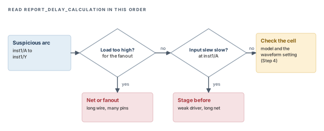
tempus> report_delay_calculation -from inst1/A -to inst1/Y ;# slew and load usedAssume it reports a load of 0.012 pF. That is the wire capacitance plus the receiver pins. Now compare it with what you expect:
- If the load is much higher than expected, the cause is the net or the fanout, not the cell.
- If the input slew is much slower than expected, look at the stage before.
- If both look normal, the cell model itself, or the waveform handling, is the next suspect.
Figure 15 shows this reading order as a decision flow. It is the same order as in Section 3.4: inputs first, result last.
Step 4 – check the waveform effect
The library team confirms the ECSM library meets the checklist in Figure 10. Thus, we enable propagation and compare.
tempus> set_delay_cal_mode -equivalent_waveform_model propagation   ;# real waveforms
tempus> report_delay_calculation -from inst1/A -to inst1/Y          ;# compare the arc
tempus> report_timing -net                                           ;# compare the path
If the delay changes noticeably, the waveform tail was affecting this stage. Keep propagation for signoff, and budget about 15% more runtime. If nothing changes, the waveform shape was not the cause, and the load or slew from Step 3 deserves a closer look.
The numbers in this example are illustrative. The method is the point: path first, then the arc, then the settings.
9 Common mistakes and how to catch them
Table 2 gathers the mistakes from this chapter. Each row starts from the symptom you would see first.
| Symptom | Likely cause | Fix |
|---|---|---|
| Delays differ from a previous run with the same data | set_design_mode -process set late or not at all |
Make it the first command of the script |
propagation gives almost no change |
Library lacks pin-cap points or real driver waveforms | Check the library against Figure 10 |
| Accuracy worse than expected at 16nm or below | Wrong pin-cap piece model or ECSM range | Confirm 8-piece ECSM, 2-piece CCS, 2%–98% range |
| A cell delay is negative | Slow input edge, fast output edge | Not an error; check both slews |
| Net delays missing from the report | -net not used |
Run report_timing -net |
| Report has the wrong columns | report_timing_format not set |
Set hpin cell slew delay arrival |
| Some delays ignore new parasitics | Arcs annotated by read_sdf |
Remove the SDF or regenerate it |
| One stage is slow, cell looks normal | Large load from a long wire or high fanout | Check the load in report_delay_calculation |
| Results poor on every setting | Library content is the limit | Review the library before tuning settings |
10 Interview preparation
A cell delay runs from a cell's input pin to its output pin. A net delay runs from a driver pin to one receiver pin.
- Cell delay depends on input slew and output load.
- Each receiver on a net has its own net delay, because it sits at a different point of the wire.
- Far receivers see later and slower edges.
Input slew and output load.
- Each table entry was measured by simulation when the library was built.
- If the point is not in the table, the tool interpolates between entries.
- A second table gives the output slew in the same way.
They store the real output waveform, so the tool can model curved edges accurately.
- CCS stores current over time; ECSM stores voltage over time.
- A simple table stores only a delay and one slew number, which assumes a straight ramp.
set_design_mode -process come first in a script?It sets node-based defaults, which should be in place before the design is loaded.
- Setting it late can make two scripts with the same data give different delays.
report_timing and report_delay_calculation?report_timing shows a whole path; report_delay_calculation explains one arc's delay.
- Use
-fromand-topins to pick the arc. - The arc report shows the input slew and load that were used, which is where most answers lie.
no_propagation and propagation settings of the equivalent waveform model.no_propagation uses the model without passing real waveforms on; propagation passes them from stage to stage.
no_propagation: about 10% more runtime.propagation: GBA and PBA, about 15% more runtime and about 8% more memory in GBA.- Choose
propagationfor small nodes and tight signoff.
Use report_timing -net.
- Set the columns with
set_global report_timing_format {hpin cell slew delay arrival}. - Net arcs end at input pins; cell arcs end at output pins.
Enough waveform data: at least 8 ECSM receiver pin-cap points, real pre-driver waveforms and an active NDW.
- Without NDW, the tool generates an analytic one, which is less accurate.
- At 16nm and below: ECSM 8-piece pin cap, CCS 2-piece, ECSM range 2% to 98%.
No. With a slow input edge and a fast output edge, the output can cross 50% before the input does.
- Delay is measured 50% to 50%, so the difference can be negative.
- The cell still switched only after its input started to move.
- The tool treats it as a normal result, and the path arrival is still correct.
Those arcs were annotated by read_sdf, which bypasses delay calculation.
- Annotated arcs ignore libraries, parasitics and delay settings.
- Remove or regenerate the SDF to get consistent results.
The library content: the result cannot be better than the data in the tables.
- No setting can recover data the library does not contain.
- Review the library before tuning settings.
Chapter recap
Key takeaways
- A stage has a driver cell, a net and receivers. Cell delay depends on input slew and output load.
- The wire adds a net delay per receiver and slows the edge, which slows the next cell.
- Libraries give delays through tables. CCS and ECSM store real waveforms and are preferred.
- Set
set_design_mode -processfirst, then load libraries, netlist, constraints and parasitics. - The equivalent waveform model handles curved edges.
propagationcarries them forward at extra cost. - Propagation needs rich library data, with extra rules at 16nm and below.
- A negative cell delay is normal. SDF-annotated arcs skip delay calculation.
Command recap
| Command or setting | Purpose |
|---|---|
set_design_mode -process 28 |
Set the node and its defaults; run first |
read_lib, read_verilog, set_top_module, read_sdc, read_spef |
Load the design data |
report_timing |
Report paths with delays and slack |
report_timing -net |
Include net arcs in the path |
report_delay_calculation -from -to |
Explain one arc's delay |
set_delay_cal_mode -equivalent_waveform_model no_propagation |
EWM only, about 10% more runtime |
set_delay_cal_mode -equivalent_waveform_model propagation |
Propagate real waveforms, about 15% more runtime |
set_global report_timing_format {hpin cell slew delay arrival} |
Choose report columns |
read_sdf |
Annotate delays; those arcs skip calculation |
Compact glossary
| Term | Meaning |
|---|---|
| Stage | A driver cell, its net and the receiver pins |
| Cell delay | Time from a cell's input pin to its output pin |
| Net delay | Time from a driver pin to one receiver pin |
| Slew | Time for an edge to move between two voltage thresholds |
| Load | Capacitance a cell output must charge or discharge |
| NLDM | Nonlinear delay model: tables of delay and slew only |
| CCS / ECSM | Library models that store output current or voltage waveforms |
| EWM | Equivalent waveform model: a more accurate description of a curved edge |
| NDW | Normalized driver waveform, a Liberty attribute |
| GBA / PBA | Graph-based (shared worst values per pin) and path-based (per-path) analysis |
| SDF | Standard delay format: a file of annotated delays |
Practical perspective
In real signoff, base delay problems rarely look like delay problems. They look like a path that fails by 10 ps for no clear reason. The habit that saves time is simple: path first, then the arc, then the library. Most surprises end at a load that is larger than expected, or at a library that lacks the data a setting needs.
What comes next
So far, every net was alone, with no neighbors switching nearby. Real wires run side by side and disturb each other. In the next chapter, Signal Integrity Delay Analysis, we add crosstalk on top of the base delay.