Chapter overview
No two transistors on a chip are exactly alike. A buffer on one side of the die can be a little slower than the same buffer on the other side. Two buffers side by side can also differ, because of random effects inside each transistor. Timing analysis must allow for this, or the silicon can fail.
The simplest allowance is a flat margin: make some delays a bit later and others a bit earlier. However, a flat margin is crude. Applied carelessly, it hides real violations or invents false ones. Both mistakes are expensive. A hidden violation can kill a chip. A false violation costs area, power and weeks of fixing.
This chapter builds the allowance step by step. We start with the early and late sides of every check. Then we pick an analysis mode, place latencies and derates, and give back the pessimism on shared clock paths. Finally, we make the derate depend on path depth and distance. This is called advanced on-chip variation (AOCV).
All times in this chapter are in ns unless stated otherwise. Timing analysis here means static timing analysis.
Learning objectives
- Explain which delays are late and which are early in a setup check and in a hold check.
- Select
single,bcwcoronChipVariationwithset_analysis_mode, and predict what each one times. - Apply clock source latency with the right
-early,-late,-minand-maxflags for each mode. - Map each OCV derate to the data, launch clock or capture clock path.
- Calculate a CPPR credit for setup and for hold, and read the
+ CPPR Adjustmentline in a report. - Describe an AOCV table, its table IDs, and how stage count and distance select a value.
- Load AOCV tables for one corner or for an MMMC library set, and enable AOCV analysis.
- Combine AOCV and user derates in multiplicative and additive modes, including reference points.
- Report AOCV derates, stage counts and arc properties in GBA and PBA.
Chapter roadmap
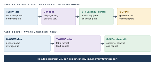
The chapter has two parts. Part A uses one flat variation factor everywhere. Part B makes that factor depend on how deep and how long a path is. Figure 1 shows the order. Come back to it whenever you lose your place.
Key commands
Table 1 lists the commands and settings in this chapter, grouped by section. Do not try to memorize them now. Each one is explained where it is first needed.
| Section | Command or setting | What it does |
|---|---|---|
| 2 Analysis types | set_analysis_mode -analysisType -checkType |
Selects single, bcwc or on-chip variation, and setup or hold |
| 2 Analysis types | report_timing -late, report_timing -early |
Reports setup (late) or hold (early) paths |
| 3 Source latency | set_clock_latency -source -early/-late -min/-max |
Sets source latency for each side of the check |
| 4 Derates | set_timing_derate -early/-late -clock/-data |
Scales delays on one side of the check |
| 5 CPPR | set_analysis_mode -cppr true |
Removes common path pessimism |
| 5 CPPR | timing_cppr_threshold_ps and eight other CPPR globals |
Fine-tune CPPR behavior |
| 7 AOCV setup | read_lib -aocv, create_library_set -aocv, update_library_set -aocv |
Load AOCV tables |
| 7 AOCV setup | set_analysis_mode -aocv true |
Turns AOCV analysis on |
| 8 AOCV control | timing_aocv_derate_mode, timing_derate_aocv_reference_point, timing_derate_ocv_reference_point |
Decide how AOCV and user derates combine |
| 8 AOCV control | set_timing_derate -delay_corner -add/-multiply |
Corner-wide and per-cell user derates |
| 8 AOCV control | timing_aocv_analysis_mode, timing_aocv_use_cell_depth_for_net |
Decide how stage depth is counted |
| 9 Reporting | report_timing -retime aocv, -retime aocv_path_slew_propagation |
Path-based AOCV reports |
1 Early and late: the two sides of every check
1.1 The concept
Every timing check compares two times at the capturing flip-flop. The first is when the data arrives. This is the arrival time. The second is the latest (or earliest) moment the data is allowed to arrive. This is the required time, and it comes from the capture clock edge.
Variation can push both times around. A slow cell makes data arrive later. A slow clock buffer makes the capture edge arrive later. The tool cannot know which way each cell will go on a real die. So it assumes the combination that hurts the check most.
Thus, every delay in a check is used on one of two sides:
- Late – the slowest value the delay could have.
- Early – the fastest value the delay could have.
Think of a train and a platform gate. If you want to know whether a passenger always catches the train, you assume the slowest walk and the earliest departure. That pairing is exactly what the tool does with late and early delays.
1.2 Why it matters
If the tool used one value for every delay, it would assume that all cells vary together. Real dies do not behave that way. One path can be slow while its neighbor is fast. Without early and late values, a design can pass analysis and still fail in silicon. Thus, every signoff check needs both sides.
1.3 How setup uses them
A setup check fails when data arrives too late for the next capture edge. So the worst case is:
- A late launch clock – the data leaves FF1 as late as possible.
- A late data path – the data travels as slowly as possible.
- An early capture clock – the next edge closes the window as soon as possible.
Let us consider Figure 2. The clock period is 2.0 ns.
- The launch clock reaches FF1 late, at 0.63.
- The late data path – clock-to-Q plus the logic – then takes 1.86. So data reaches FF2/D at 0.63 + 1.86 = 2.49.
- The capture clock reaches FF2 early, at 2.00 + 0.57 = 2.57.
- The setup time of FF2 is 0.10. So the required time is 2.57 − 0.10 = 2.47.
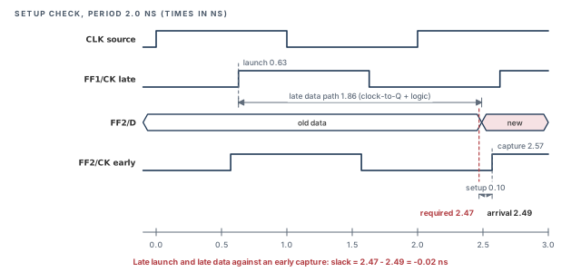
For setup, slack is required minus arrival. Here it is 2.47 − 2.49 = −0.02 ns. Keep these numbers in mind. We will return to them when we remove pessimism in section 5.
1.4 How hold uses them
A hold check fails when new data arrives too soon and corrupts the value being captured. It compares the launch and capture of the same clock edge. So the worst case is the reverse of setup:
- An early launch clock – new data leaves FF1 as soon as possible.
- An early data path – it races through the logic.
- A late capture clock – FF2 still needs the old value for a while.
Let us use the same clock tree with a second, very short path from FF1 to FF2. Figure 3 shows the numbers.
- The launch clock reaches FF1 early, at 0.57.
- The short data path takes 0.10 at its early value. So new data reaches FF2/D at 0.67.
- The capture clock reaches FF2 late, at 0.63.
- The hold time of FF2 is 0.05. So the data must not change before 0.63 + 0.05 = 0.68.
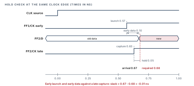
For hold, slack is arrival minus required: 0.67 − 0.68 = −0.01 ns. We will fix this one with CPPR as well.
A beginner swaps the formulas and reads a failing hold path as passing. Remember the direction. Setup slack is required minus arrival. Hold slack is arrival minus required. In both cases, a negative number is a violation.
2 The three analysis types
2.1 The concept
The tool needs to know where its early and late values come from. Should both come from one library? Should setup use a slow library and hold a fast one? Or should one library be scaled up and down inside the same check? The analysis type answers this question.
The command is set_analysis_mode. Its two options for this purpose are shown below.
tempus> set_analysis_mode \
          -analysisType {single | bcwc | onChipVariation} \
-checkType {setup | hold}-analysisType– where early and late delays come from. The three values are explained in the next subsections.-checkType– which check the session times:setuporhold. It is most useful insinglemode, where it is one of two ways to time hold.
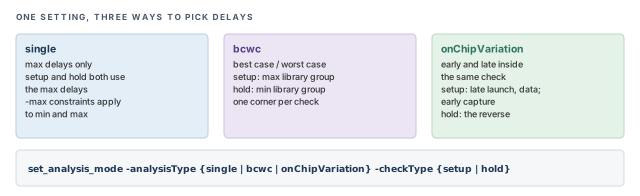
Figure 4 compares the three types side by side.
2.2 single
In single mode, the tool uses max delays only. There is no second library group and no early copy of each delay. Constraints given with -max apply to both min and max analysis. For example, an input delay set only with -max is also used when the tool times hold.
To time hold in single mode, use either of these two methods:
tempus> set_analysis_mode -analysisType single -checkType hold   ;# switch to hold
tempus> report_timing -early                                      ;# or ask for early paths
Single mode is useful for quick checks, for example early in a block's life. It is fast and simple. However, it cannot show what happens when two paths on one die vary differently.
2.3 bcwc
bcwc stands for best case, worst case. Setup uses the max library group, usually the slow corner. Hold uses the min library group, usually the fast corner. Each check therefore sees one corner at a time.
Let us consider what this means. In a bcwc setup check, the launch clock, the data and the capture clock all use slow delays. The whole die is assumed to be slow together. This is a fair picture of global process shifts. However, it does not cover a slow launch path next to a fast capture path.
2.4 onChipVariation
In onChipVariation (OCV) mode, early and late values are used inside the same check. This is the mode that matches Figures 2 and 3. It is the usual signoff mode, because it covers variation between two paths on the same die.
In OCV mode, report_timing -late reports setup paths. report_timing -early reports hold paths.
Table 2 sums up the three types.
| Type | Setup uses | Hold uses | Covers on-die variation? |
|---|---|---|---|
single |
Max delays | Max delays (via -checkType hold or -early) |
No |
bcwc |
Max library group | Min library group | No – one corner per check |
onChipVariation |
Late launch and data, early capture | Early launch and data, late capture | Yes |
Figure 5 shows the same comparison for one setup check, segment by segment. Read each row from left to right. In single and bcwc, all three segments use the same kind of delay. Only onChipVariation lets the two clock paths take opposite sides.
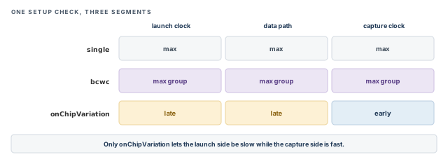
A beginner runs single mode for signoff and sees few violations. The reason is that no early-against-late variation was applied. Use onChipVariation when you need on-die variation in the check.
single uses max delays only, bcwc uses one library group per check, and onChipVariation puts early and late into the same check.3 Clock source latency in each mode
3.1 The concept
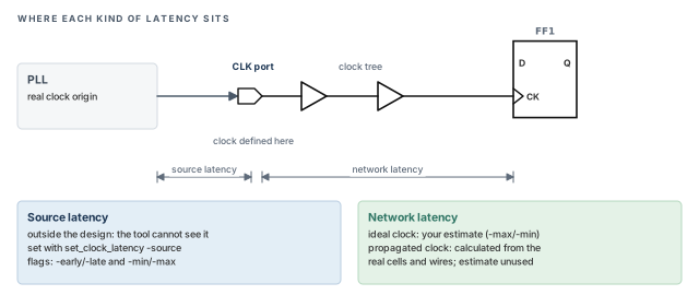
A clock does not start at the clock pin of your block. It starts at a real origin, such as a PLL or an oscillator. Source latency is the delay from that real origin to the point where the clock is defined. It is outside the design, so the tool cannot calculate it. The designer gives it with set_clock_latency -source.
Source latency also varies. The PLL output and the top-level routing can be a little faster or slower. So the designer usually gives more than one value. Each value can carry two kinds of flags:
-earlyor-late– which side of the check the value is for.-minor-max– which library group the value belongs to.
Figure 6 shows where source latency ends and network latency begins. Network latency is the delay through the clock tree inside the design. We return to it at the end of this section.
3.2 How the mode picks a value
The tool picks a value by both flags, as Table 3 shows. In bcwc, both flags are needed. In OCV, the side of the check decides, and the min/max flag is optional – shown in brackets.
| Mode | Setup launch | Setup capture | Hold launch | Hold capture |
|---|---|---|---|---|
| bcwc | -source -late -max |
-source -early -max |
-source -early -min |
-source -late -min |
| onChipVariation | -late [-max] |
-early [-min] |
-early [-min] |
-late [-max] |
Let us read the bcwc row slowly. Setup reads only -max values, because setup uses the slow library group. Within that group, launch still takes the late value and capture the early value. Hold reads only -min values, and swaps the sides. Thus, in bcwc, a setup check never sees a -min latency, and a hold check never sees a -max latency.
In OCV, the logic is simpler. The side of the check decides: launch is late for setup and early for hold.
3.3 Practical example
Assume the PLL output can arrive between 0.30 and 0.36 ns after the reference edge.
tempus> set_clock_latency -source -late -max 0.36 [get_clocks CLK]   ;# slowest arrival
tempus> set_clock_latency -source -early -min 0.30 [get_clocks CLK]  ;# fastest arrival
For setup, the launch clock then starts 0.36 after the edge and the capture clock 0.30 after it. This difference of 0.06 ns reduces the setup slack. Figure 7 draws this with an assumed period of 2.0 ns.
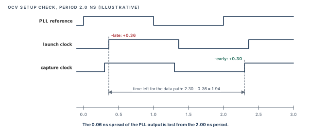
For hold, the two values swap, and the same 0.06 ns reduces the hold slack.
These two lines are enough for OCV. A bcwc session needs two more values, as Table 3 shows. It needs -source -early -max for setup capture and -source -late -min for hold capture.
3.4 Network latency on ideal clocks
Network latency is the delay inside the design, through the clock tree. Before clock tree synthesis, there is no tree yet. The clock is ideal, and the designer estimates the tree delay with a network latency value.
Note that the -max and -min network latency values apply only to ideal clocks. Once a clock is propagated, the tool calculates the real tree delay from the cells and wires. The estimate is then no longer used.
After clock tree synthesis, a designer edits the network latency and sees no change in the report. Nothing is broken. The clock is propagated, so the tool uses the real tree delay instead.
-max/-min latency only affects ideal clocks.4 OCV derates: which flag goes on which path
4.1 The concept
A derate is a factor that scales a delay. A late derate of 1.05 makes a 0.40 ns delay 0.42 ns. An early derate of 0.95 makes the same delay 0.38 ns. In OCV mode, derates create the early and late values used in Figures 2 and 3.
Where does the factor come from? Usually the library or methodology team measures how much delays spread on silicon. They turn that spread into a factor, such as ±5 %. The designer then applies it with set_timing_derate.
4.2 How the derates map to the check
set_timing_derate takes a side (-early or -late) and a path type (-clock or -data). Table 4 shows which pair applies to each path. Figure 8 puts the same mapping onto the circuit.
| Check | Data path | Launch clock path | Capture clock path |
|---|---|---|---|
| Setup | -late -data |
-late -clock |
-early -clock |
| Hold | -early -data |
-early -clock |
-late -clock |
Thus, one set of four derates covers both checks. The tool picks the right one for each segment and each check. For example:
tempus> set_timing_derate -late -clock -cell_delay 1.05    ;# slow clock cells
tempus> set_timing_derate -early -clock -cell_delay 0.95   ;# fast clock cells
tempus> set_timing_derate -late -data -cell_delay 1.05     ;# slow data cells
tempus> set_timing_derate -early -data -cell_delay 0.95    ;# fast data cells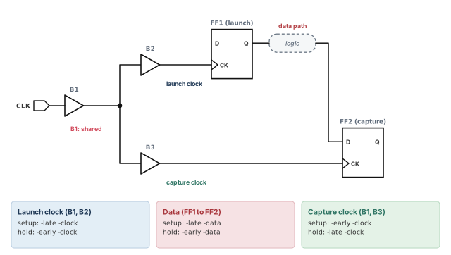
4.3 Command breakdown
-late/-early– the side of the check this factor feeds. A late factor is normally above 1.0. An early factor is normally below 1.0. Mixing them up makes the analysis optimistic.-clock/-data– the kind of path the factor applies to. Clock paths are the launch and capture clock networks. Data paths run from the launch flop to the capture pin.-cell_delay– the factor applies to cell delays. The value is the factor itself, such as 1.05.-delay_corner– in an MMMC session, limits the derate to one corner. We return to delay corners in Multi-Mode Multi-Corner Analysis. Section 8 shows this option in use.
It is better to derate the clock and data paths separately, even when the values start out equal. The reason is that the clock tree is often built from different cells. You will want to tune it alone later, without touching the data paths.
5 Removing common path pessimism (CPPR)
5.1 The concept
Let us look again at our circuit, now with the clock tree drawn out in Figure 9. Buffer B1 drives both flip-flops. It sits on the launch clock path and on the capture clock path. Its nominal delay is 0.40 ns.
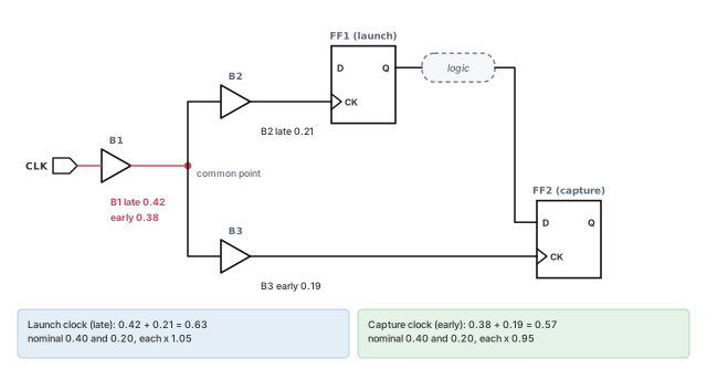
In the setup check, B1 is taken late (0.42) for launch and early (0.38) for capture. However, one buffer cannot be slow and fast at the same moment. Both clock edges pass through the same transistors, at most one clock cycle apart. The buffer cannot change its speed in that short time. The 0.04 ns difference is therefore not real. It is called common path pessimism.
The point where the launch and capture clock paths split is the common point. Everything before it is the common path.
5.2 Why it matters
Common path pessimism grows with the shared part of the tree. In a large design, the shared trunk can be long. Then every flop pair under it carries a false penalty. Without removal, the tool reports violations that do not exist. Engineers then fix them by adding buffers or upsizing cells, which wastes area and power.
5.3 How CPPR works
Common path pessimism removal (CPPR) gives this false penalty back. The tool works in three steps:
- It finds the common point of the launch and capture clock paths.
- It adds up the late-minus-early delay of every cell and net before that point.
- It adds this sum to the slack as a credit.
For our setup check, the credit is 0.42 − 0.38 = 0.04 ns. The slack becomes −0.02 + 0.04 = +0.02 ns. Figure 10 shows the effect.
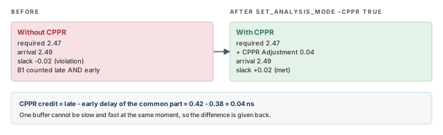
The same credit applies to hold. In the hold check, B1 is taken early (0.38) for launch and late (0.42) for capture. The difference is again 0.04 ns. So the hold slack of −0.01 ns becomes +0.03 ns.
5.4 Command breakdown
The command is simple:
tempus> set_analysis_mode -cppr true ;# remove common path pessimism- In the report, the credit appears as a separate line labeled
+ CPPR Adjustment. The arrival and required times stay as they were. - CPPR works in all analysis modes, not only in OCV.
- It also handles reconvergent clock paths – clock paths that split and meet again before reaching a flop.
5.5 The CPPR globals
Nine globals adjust CPPR. Table 5 lists them, with what each name refers to. These descriptions are read from the names. Check the exact meaning, values and defaults with help before changing any of them.
| Global | What the name refers to |
|---|---|
timing_cppr_threshold_ps |
A tolerance in ps: pessimism below it may be left in place (default 20 ps) |
timing_cppr_remove_clock_to_data_crp |
Credit where a clock path feeds a data path |
timing_cppr_self_loop_mode |
Paths that launch and capture at the same flop |
timing_cppr_skip_clock_reconvergence |
Whether reconvergent clock paths are analyzed |
timing_enable_pessimistic_cppr_for_reconvergent_clock_paths |
A safer, more pessimistic credit on reconvergent clocks |
timing_cppr_transition_sense |
How rise and fall transitions are matched on the common path |
timing_enable_si_cppr |
CPPR on signal integrity delay changes |
timing_cppr_opposite_edge_mean_scale_factor |
Credit scaling when launch and capture use opposite edges (mean part) |
timing_cppr_opposite_edge_sigma_scale_factor |
The same scaling, for the sigma part of statistical delays |
The default threshold is 20 ps. Thus, up to 20 ps of pessimism can remain on a path, even with CPPR on. Our 40 ps example is well above the threshold. A shared-path difference of only 15 ps might not be given back. Do not assume a path with CPPR is free of all pessimism.
When a few picoseconds decide whether a path passes, look at the shared clock path first. A small leftover within the threshold is a common reason for a near-miss.
6 AOCV: derates that depend on depth
6.1 The concept
A flat derate assumes every path varies by the same percentage. However, random variation does not behave that way. Think of tossing coins. One coin gives all heads or all tails. A hundred coins almost always give close to half and half. The random errors cancel.
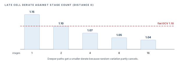
Cells behave in a similar way. On a long chain, some cells are a little fast and others a little slow. They partly cancel. Here is a rough guide. Suppose each cell varies by about ±10 %. A chain of 16 similar, independent cells then varies by about ±10 % / √16 = ±2.5 % of its total delay. So a deep path varies by a smaller percentage than a single cell.
Advanced on-chip variation (AOCV) uses this fact. Its derate shrinks as the number of stages grows. A stage is one cell along the path, together with the net it drives.
6.2 Why it matters
A flat derate must be large enough to protect the shortest paths. Suppose the flat late derate is 1.10. Then every long data path carries far more margin than it needs. The tool reports violations that silicon would not show. Engineers upsize cells that never needed it.
AOCV removes this waste. It is also more honest about short paths. A one-stage path may get a derate above the flat value. Figure 12, after the next subsection, shows an illustrative late table against a flat OCV derate of 1.10.
6.3 Distance as a second axis
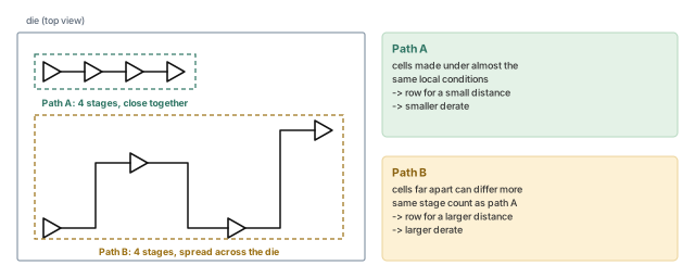
Variation also grows with distance. Two cells next to each other were made under almost the same conditions. Two cells at opposite corners of a large die may differ more. So an AOCV table can have a second axis: distance in microns. Each row is one distance and each column one stage count.
Figure 11 compares two paths with the same four stages. Path A sits in one small area. Path B is spread across the die. The stage count is equal, so only distance tells them apart.
Thus, the derate goes down with more stages and up with more distance. A deep, compact path gets the smallest derate. A shallow path spread across the die gets the largest.
6.4 How the tool counts stages
The tool counts the stages along each path. The count is taken differently in the two analysis styles:
- Graph-based analysis (GBA) – the default style. It times each pin once, with the worst values from all paths through it. In GBA, AOCV uses stage count only. The distance row is chosen from the chip or core size.
- Path-based analysis (PBA) – re-times one path at a time, with the exact values of that path. It is slower but less pessimistic.
The chip or core size for GBA comes from the physical data, when it is loaded. Without physical data, the settings aocv_chip_size and aocv_core_size give it.
The clock path count also differs. In GBA, the count restarts at every clock branch point. In PBA, it starts at the CPPR common point of the launch and capture pair. Figure 13 shows why GBA is the more pessimistic of the two.
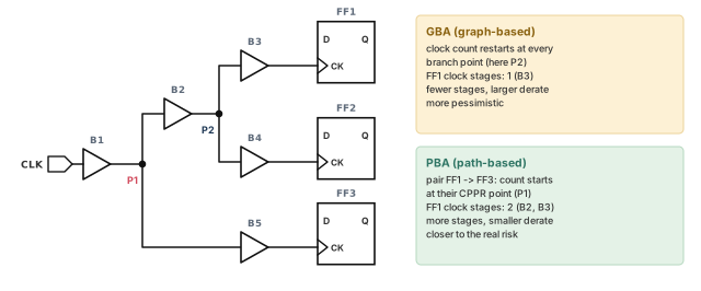
Let us walk through Figure 13. The pair is FF1 (launch) and FF3 (capture). Their clock paths split at P1, so P1 is their common point. PBA counts the FF1 clock path from P1: B2 and B3, two stages. GBA cannot look at one pair at a time. It restarts at every branch point, so it counts from P2: only B3, one stage. One stage reads a larger derate from the table than two stages.
7 Setting up AOCV
7.1 The AOCV table format
AOCV tables use the Cadence format. Table 6 lists its fields.
| Field | Meaning |
|---|---|
Apply-Net / Apply-Cell |
Optional: whether the table applies to nets or cells |
Voltage |
The supply voltage of the table; values between voltages are interpolated, values outside are clamped |
| Table ID | Which delays the table covers, for example Late-Rise-Data (pattern below) |
| Object ID | A library or library cell only, for example Cell stdcell/* |
Stage |
The stage-count axis (columns) |
Distance |
Optional distance axis in microns (rows) |
The Voltage field deserves a short example. Suppose tables exist for 0.80 V and 0.90 V, and a cell runs at 0.85 V. The tool interpolates between the two tables. If the cell runs at 0.95 V, outside the range, the tool clamps to the 0.90 V table.
The Object ID names what the table applies to. It can be a library or a library cell, for example Cell stdcell/* for every cell in the library stdcell. It cannot be an instance in your design.
A table ID follows this pattern. Braces list the choices and square brackets mark optional parts.
{Early|Late}[-{Rise|Fall}][-{Clock|Data}]Three rules about table IDs matter in practice:
- Both Early and Late tables are required. Early tables feed the fast side of each check, and Late tables the slow side.
- The rise/fall and clock/data parts are optional. A plain
Latetable covers every late delay. - When several tables match a delay, the most specific one wins. For example,
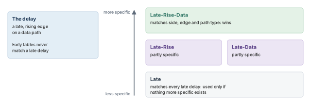
Late-Rise-DatabeatsLatefor a rising data delay.
Figure 14 shows rule 3 for one delay: a late, rising edge on a data path. Four tables could match it. The tool uses the one that names the most details.
7.2 Lookup and range
Figure 15 shows a lookup. Stage count picks the column and distance picks the row. A 4-stage path at 1000 µm reads 1.10 from the table.
When a stage count or distance is outside the table, the tool uses the last value in that direction. It never extrapolates.
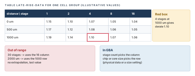
On the stage axis, clamping errs on the safe side. A deeper path would vary even less, so reusing the last column keeps a little extra margin. On the distance axis, the opposite holds. A path longer than the last row may vary more than the table says. Thus, make sure the distance rows cover the largest distance in your design.
7.3 Loading and enabling AOCV
First turn AOCV on. Then load the tables. For a single-corner session, use read_lib -aocv:
tempus> set_analysis_mode -aocv true            ;# enable AOCV analysis
tempus> read_lib -aocv "myDerateLib.aocv.lib"   ;# load the AOCV tables
In an MMMC session, the tables belong to a library set. Attach them when you create the set, or add them to an existing set:
tempus> create_library_set -name slow -timing slow.lib -aocv test.aocv.lib   ;# new set
tempus> update_library_set -name slow -aocv test.aocv.lib ;# existing set-name– the library set to create or update.-timing– the timing libraries of the set.-aocv– the AOCV table files for this set.
Note that -aocv and -socv are mutually exclusive on one library set. Statistical tables are the subject of SOCV and Wire Variation.
Loading the tables without set_analysis_mode -aocv true leaves the analysis on flat derates. The report then looks normal but shows no AOCV columns. Check for the aocv_derate column after the first run.
8 Combining and controlling AOCV derates
8.1 AOCV derates and user derates together
Many flows keep a small user OCV derate on top of AOCV. It covers effects the tables do not model, such as an extra margin set by the methodology team. The tool must then combine two numbers for each delay: the AOCV derate X and the user derate Y.
The global timing_aocv_derate_mode decides how:
aocv_multiplicative– the default. The result is X × Y. For example, 1.07 × 1.02 = 1.0914.aocv_additive– the result is a sum, adjusted by two reference points.
8.2 Reference points
The globals timing_derate_aocv_reference_point and timing_derate_ocv_reference_point each take 0 or 1. The default is 1 for both. The first applies to the AOCV value X, the second to the user value Y.
In additive mode the formulas are:
- Both reference points 1: X + Y − 1.
- One reference point 0: X + Y.
- Both reference points 0: X + Y + 1.
One way to read these formulas is this. A reference point of 1 means the derate is written as a factor near 1, such as 1.02. A reference point of 0 means it is written as a change near 0, such as 0.02. The formulas then simply undo the extra "1" each factor carries. Figure 16 works all four cases with the same numbers.
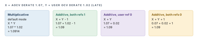
A designer selects additive mode, keeps both reference points at 0, but writes the derates as factors (1.07 and 1.02). The result is 1.07 + 1.02 + 1 = 3.09, a huge derate. Always write the values in the form the reference points expect.
8.3 Corner and per-cell user derates
set_timing_derate can also target one corner and one set of cells. The first line below sets a late cell derate for the whole dcMax corner. The second adds an extra 0.02 on one instance.
tempus> set_timing_derate -delay_corner dcMax -late -cell_delay 1.01   ;# whole corner
tempus> set_timing_derate -delay_corner dcMax -late -cell_delay 0.02 \
-add [get_cells U1] ;# add 0.02 on U1-delay_corner dcMax– limits the derate to the delay corner nameddcMax.-add– the value is added to the existing derate of the listed cells.-multiply– the value scales the existing derate instead. Use it when the extra margin is a factor, not a step.
Assume -add stacks on the corner value. Then U1 sees 1.01 + 0.02 = 1.03 as its late user derate, before AOCV is combined.
8.4 How stages are counted
Two more globals control the stage count:
timing_aocv_analysis_mode– takescombine_launch_capture,launch_capture,clock_onlyorseparate_data_clock. It decides how launch, capture, clock and data stages form the count. The names suggest which parts are counted together; confirm each value withhelp.timing_aocv_use_cell_depth_for_net– defaultfalse. From its name, it decides whether net derates use the cell depth of the path; confirm withhelp.
Do not rely on a remembered default for timing_aocv_analysis_mode. Both launch_capture and combine_launch_capture have been described as the default. Confirm it in your installation with get_global timing_aocv_analysis_mode, and set it explicitly in your scripts.
9 Reporting AOCV
9.1 Choosing the report
Three forms of report_timing show AOCV results. Table 7 compares them. Each step down the table is slower but less pessimistic.
| Command | Style | Stage count | Slew |
|---|---|---|---|
report_timing |
GBA | Graph-based count | Graph-based slew |
report_timing -retime aocv |
PBA | Path-based count | Graph-based slew |
report_timing -retime aocv_path_slew_propagation |
PBA | Path-based count | Path-based slew |
-retime aocv– re-times the reported path with its own stage count.-retime aocv_path_slew_propagation– also re-propagates the slews along that one path. Slews then come from this path only, not from the worst of all paths through each pin.
9.2 Columns and properties
Three report columns show the AOCV numbers: aocv_derate, user_derate and stage_count. One way to show them is to add them to the report format, as below. Confirm the exact column names with help report_timing in your installation.
tempus> set_global report_timing_format \
          {hpin cell delay aocv_derate user_derate stage_count arrival}   ;# show AOCV
tempus> report_timing -retime aocv                                      ;# PBA count
When reading the report, note that pin rows show a derate of 1.000. Only the arc rows carry the real derate. Thus, look at the cell and net arc rows.
The same values are stored as arc properties. Their names follow a fixed pattern, for example aocv_stage_count_data_late and aocv_derate_capture_clock_early_rise. Scripts can read them with get_property, for example to list every arc whose derate exceeds a limit.
Use plain report_timing to find candidates, then -retime aocv_path_slew_propagation on the worst paths. The reason is runtime: path-based retiming is slower but less pessimistic.
-retime aocv and -retime aocv_path_slew_propagation tighten the count and the slew. Read derates on arc rows, not pin rows.10 Worked example: from flat OCV to AOCV
The task. A block fails setup by 0.02 ns on the path in Figure 9. The team suspects pessimism rather than a real problem. The team also plans to move from flat derates to AOCV tables. We will do both, step by step, and check each number.
Step 1 – OCV mode with flat derates
We first reproduce the failure, so that every later change can be measured against it.
# Assuming one setup corner, times in ns, flat 5 percent derates
tempus> set_analysis_mode -analysisType onChipVariation -checkType setup   ;# OCV
tempus> set_timing_derate -late -clock -cell_delay 1.05    ;# launch clock slow
tempus> set_timing_derate -early -clock -cell_delay 0.95   ;# capture clock fast
tempus> set_timing_derate -late -data -cell_delay 1.05     ;# data slow
tempus> report_timing -late                                ;# setup paths
The slack is −0.02, as in Figure 2. In the report, B1 appears twice. It shows 0.42 on the launch clock and 0.38 on the capture clock.
Step 2 – remove common path pessimism
tempus> set_analysis_mode -cppr true   ;# give back the common part
tempus> report_timing -late            ;# look for + CPPR Adjustment
The report now shows + CPPR Adjustment of 0.04, and the slack becomes +0.02. The 0.02 ns violation was pessimism on buffer B1. The 40 ps credit is well above the 20 ps threshold, so the threshold does not affect this path.
Step 3 – depth-aware derates
Now the team switches to the AOCV tables from the library team. It keeps a small user derate of 1.02 for late data, which replaces the flat 1.05.
tempus> set_analysis_mode -aocv true                          ;# enable AOCV
tempus> update_library_set -name slow -aocv blkA.aocv.lib     ;# attach tables
tempus> set_timing_derate -late -data -cell_delay 1.02        ;# small user derate
tempus> get_global timing_aocv_derate_mode                    ;# expect multiplicative
tempus> get_global timing_aocv_analysis_mode                  ;# confirm, do not assume
tempus> report_timing -retime aocv_path_slew_propagation ;# PBA count and slewhpin cell delay aocv_derate user_derate stage_count
U7/Y BUFX2 0.214 1.070 1.020 4Step 4 – check the numbers by hand
The data path has 4 stages. Assume its cells sit close together, so the 0 µm row of the table applies: the AOCV derate is 1.07. The user derate is 1.02. In multiplicative mode the cell delay is scaled by 1.07 × 1.02 = 1.0914.
Assume the BUFX2 delay is 0.196 ns before derating. Then 0.196 × 1.0914 ≈ 0.214 ns, which matches the report row.
Step 5 – compare with the flat derate
Before AOCV, this cell took the flat 1.05. Now it takes 1.0914, which is larger. So this short, 4-stage path gets worse under AOCV, not better.
This is not an error. AOCV is not a slack giveaway; it moves margin to where the variation really is. Shallow paths get more margin, and deep paths get less.
The flat 1.05 in this block was already aggressive. A 16-stage path reads 1.04 × 1.02 ≈ 1.061, which is still above 1.05. Against a more conservative flat derate such as 1.10, however, deep paths clearly gain.
Figure 17 puts every column of the 0 µm row next to both flat values. Each bar is the AOCV value times the user derate of 1.02.
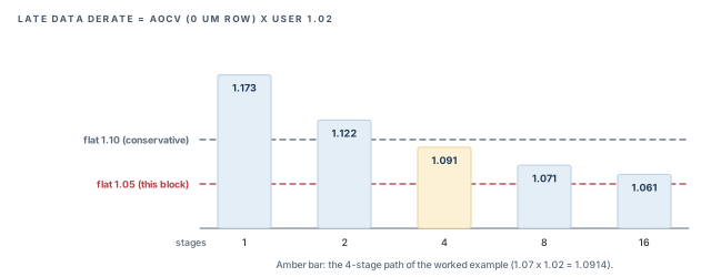
After any switch from flat derates to AOCV, re-check short paths as well as long ones. Short paths are where new violations usually appear.
11 Common mistakes and how to catch them
Table 8 gathers the mistakes from this chapter. Each row gives the symptom you would see first.
| Symptom | Likely cause | Fix |
|---|---|---|
| Hold looks clean in single mode | Only max delays are used | Use -checkType hold or report_timing -early; use OCV for signoff |
| Hold uses setup latency values | Latency flags do not match the mode | Give each value the early/late and min/max flags its mode needs |
| Network latency ignored after CTS | Clock is propagated | -max/-min network latency only applies to ideal clocks |
| Optimistic results with OCV | Early and late derates swapped | Late factors above 1.0, early factors below 1.0 |
| Setup or hold fails by a few ps on shared clocks | CPPR is off | set_analysis_mode -cppr true |
| Small pessimism remains with CPPR on | Leftover within timing_cppr_threshold_ps (20 ps) |
Expected; adjust the threshold only with care |
No aocv_derate column values |
AOCV not enabled | set_analysis_mode -aocv true |
| Table set fails review | Only Late tables were written | Both Early and Late tables are required |
| Derate much larger than expected | GBA count restarted at a clock branch | Retime with -retime aocv |
| Derate of 1.000 everywhere in the report | Reading pin rows | Read the arc rows |
| Additive derate near 3.0 | Reference points do not match how values are written | Set the reference points to 1 for factors, 0 for changes |
| Short paths fail after moving to AOCV | Shallow paths get large AOCV derates | Expected; check and fix them like any real violation |
| Stage counts differ between two flows | timing_aocv_analysis_mode differs between scripts |
Set it explicitly in every script |
12 Interview preparation
The launch clock and data are late; the capture clock is early.
- This makes data arrive as late as possible and the window close as soon as possible.
- Hold is the reverse: early launch and data, late capture.
bcwc and onChipVariation?bcwc uses one library group per check; OCV mixes early and late values within one check.
- bcwc: setup from the max group, hold from the min group.
- bcwc assumes the whole die is slow or fast together. OCV also covers two paths varying differently on one die.
Use set_analysis_mode -checkType hold, or report_timing -early.
- Single mode uses max delays only.
-maxconstraints apply to both min and max analysis in this mode.
The value set with -source -late -min.
- Hold reads
-minvalues, because hold uses the min library group. - Capture is the late side for hold, because a late capture edge hurts hold.
-early -clock.
- An early capture edge closes the setup window sooner, which is the worst case.
- For hold, the capture clock uses
-late -clock.
It removes the pessimism of using one shared clock buffer at two different speeds in the same check.
- The credit is the late-minus-early delay of the path before the common point.
- It applies to setup and to hold.
- It appears as
+ CPPR Adjustmentin the report.
The leftover pessimism is within the CPPR threshold, which is 20 ps by default.
- The global is
timing_cppr_threshold_ps. - Up to that amount of pessimism can remain on a path.
Random variation along many stages partly cancels, so the total varies by a smaller percentage.
- Some cells are fast and others slow, like coin tosses averaging out.
- Distance works the other way: cells farther apart vary more, so the derate grows.
GBA restarts the stage count at every clock branch point; PBA counts from the pair's CPPR point.
- Fewer stages give a larger derate.
- GBA also uses stage count only, with the distance row from chip or core size.
1.09, from X + Y − 1.
- The "− 1" removes the second copy of 1.0 that both factors carry.
- Multiplicative mode, the default, would give 1.0914.
The 16-stage value; AOCV lookups never extrapolate.
- The same rule applies to distance beyond the last row.
No. Pin rows always show 1.000; the real derate is on the arc rows.
- Read the cell and net arc rows for
aocv_derate,user_derateandstage_count.
Chapter recap
Key takeaways
- Setup uses late launch and late data against early capture; hold uses the reverse.
singleuses max delays only,bcwcuses one library group per check, andonChipVariationmixes early and late in one check.- Source latency needs the flags its mode expects; network
-max/-minlatency only affects ideal clocks. - CPPR gives back the late-minus-early delay of the shared clock path, for setup and hold, down to a 20 ps threshold.
- AOCV tables lower the derate for deep paths and raise it for distant ones; lookups clamp at the table edges.
- GBA counts clock stages from each branch point; PBA counts from the pair's CPPR point.
- AOCV and user derates combine multiplicatively by default; additive mode depends on the reference points.
- AOCV can make short paths worse. Re-check them after every switch.
Command recap
| Command or setting | Purpose |
|---|---|
set_analysis_mode -analysisType -checkType |
Choose the analysis type and the check |
set_analysis_mode -cppr true |
Remove common path pessimism |
set_analysis_mode -aocv true |
Enable AOCV |
set_clock_latency -source -early/-late -min/-max |
Source latency per side and group |
set_timing_derate -early/-late -clock/-data |
Flat OCV derates |
set_timing_derate -delay_corner -add/-multiply |
Corner and per-cell derates |
read_lib -aocv, create_library_set -aocv, update_library_set -aocv |
Load AOCV tables |
timing_aocv_derate_mode, timing_derate_*_reference_point |
How AOCV and user derates combine |
timing_aocv_analysis_mode, timing_aocv_use_cell_depth_for_net |
How stages are counted |
report_timing -retime aocv, -retime aocv_path_slew_propagation |
Path-based AOCV reports |
Compact glossary
| Term | Meaning |
|---|---|
| Arrival / required time | When data arrives / when it must arrive by (setup) or not before (hold) |
| Early / late | The fastest / slowest value a delay is assumed to take |
| bcwc | Best case, worst case: one library group per check |
| OCV | On-chip variation: early and late values in the same check |
| Derate | A factor that scales a delay up or down |
| Source latency | Clock delay from the real origin to the clock definition point |
| Network latency | Clock delay through the clock tree inside the design |
| Common point | The last point shared by the launch and capture clock paths |
| CPPR | Common path pessimism removal: the credit for the shared clock path |
| AOCV | Advanced on-chip variation: derates by stage count and distance |
| Stage count | The number of cell stages counted along a path |
| GBA / PBA | Graph-based / path-based analysis |
| Reference point | Whether a derate is written as a factor (1) or a change (0) |
Practical perspective
On a real project, pessimism is never free. Every false violation costs an ECO, extra area or extra power. Every missing margin risks a silicon failure. Thus, a signoff engineer must be able to explain each derate on a critical path. Start from OCV with CPPR, add AOCV tables from the library team, and check short paths after every change. Most debates about "is this violation real?" end with exactly the numbers in this chapter.
What comes next
AOCV still uses fixed tables. In the next chapter, SOCV and Wire Variation, each delay carries a mean and a sigma instead. We will see how the tool adds variation statistically, and how wire resistance and capacitance can vary too.