Chapter overview
In Analysis Modes, CPPR and AOCV we pushed every cell to a worst-case delay with derates. That approach is safe, but its fixed factors act as if every cell on a path were slow at once. In real silicon, that almost never happens. Some cells are a little slow and some a little fast, and the errors partly cancel.
Statistical on-chip variation (SOCV) models this directly. Each delay becomes a mean and a sigma. The tool combines them along the path and reports a single, less pessimistic number. For deep paths, this can turn a false violation into a passing path.
The same idea extends to wires. Metal layers vary in resistance and capacitance from one chip to the next. Wire variation adds those per-layer effects to path-based analysis.
This chapter covers both, from the data files to the report fields. We also spend time on the traps. Several common inputs quietly carry no sigma, and a beginner can lose margin without noticing.
Learning objectives
- Explain mean and sigma for a cell delay, and why sigmas add as root-sum-square.
- Calculate a path arrival at n sigma, and compare it with a stage-by-stage sum.
- Describe the two sources of SOCV data – Liberty LVF and the
.socvfile – and their main attributes. - Load SOCV data for single-corner and MMMC sessions, and bootstrap it from AOCV tables for experiments.
- Turn on SOCV analysis, set the statistical min/max mode and the reporting n-sigma.
- Read SOCV report fields and timing properties, including mean and sigma values.
- List the inputs and outputs that carry no sigma, or only the mean, and avoid their traps.
- Set up wire variation with an extended SPEF, a side file and path-based reporting.
- Choose between the statistical and binomial wire variation models.
Chapter roadmap
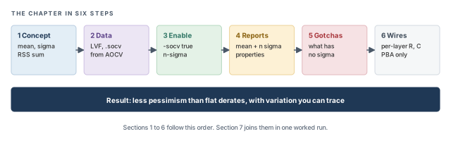
The chapter moves in six steps, from the statistical idea to per-layer wire effects. Figure 1 shows the order. Come back to it whenever you lose your place.
Key commands
Table 1 lists the commands and settings covered in this chapter, grouped by the section that teaches them. Do not try to memorize them now. Each one is explained when it is first needed.
| Section | Command or setting | What it does |
|---|---|---|
| Data | read_lib -socv, read_lib (LVF) |
Load sigma from .socv or LVF |
| Data | create_library_set -socv |
Attach .socv files in MMMC |
| Data | timing_library_infer_socv_from_aocv |
Infer sigma from AOCV (experiments) |
| Data | timing_library_scale_aocv_to_socv_to_n_sigma |
Sigma level of an AOCV value |
| Enable | set_analysis_mode -socv true |
Turn on statistical analysis |
| Enable | timing_socv_statistical_min_max_mode |
Rule for statistical max and min |
| Enable | set_socv_reporting_nsigma_multiplier |
n in mean + n × sigma for reports |
| Reports | timing_report_enable_verbose_ssta_mode |
Show mean and sigma details |
| Traps | set_timing_derate -mean, -sigma |
Derate only the mean or the sigma |
| Traps | write_sdf -no_variation |
Write mean-only delays to SDF |
| Traps | -via_variation_file |
Add via variation |
| Wires | read_spef -extended -wire_variation_file |
Read layer tags and wire variation |
| Wires | timing_enable_wire_variation |
Turn on wire variation |
| Wires | set_wire_variation_mode |
Choose the wire variation model |
| Wires | report_timing -retime path_slew_propagation |
Path-based report with wire variation |
1 From flat derates to statistics
1.1 The concept
Let us start with one cell. If we build the same cell on many chips, its delay is not one number. Tiny differences in transistor size, doping and thickness make each copy a little different. The delays spread around an average value.
The average is the mean, written μ. The spread is measured by the standard deviation, or sigma, written σ. A small sigma means most copies behave almost the same. A large sigma means the delay is hard to predict.
For example, assume a buffer has a mean delay of 100 ps and a sigma of 10 ps. Figure 2 shows the spread. About 99.7% of chips fall between μ − 3σ and μ + 3σ – here, between 70 ps and 130 ps.
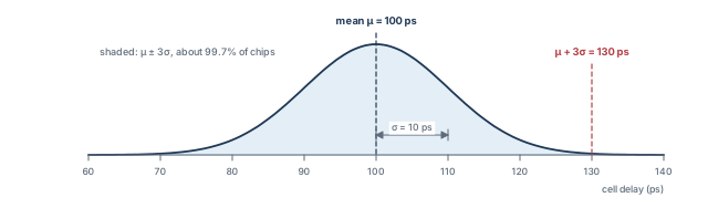
The term n sigma means mean + n × σ. At n = 3, this buffer's late delay is 100 + 3 × 10 = 130 ps. At n = 2, it is 120 ps. Thus, n is a confidence knob: a larger n covers more chips, but adds more margin.
1.2 A picture from daily life
Think of a trip to work in three legs: a bus, a train and a short walk. Each leg usually takes about 10 minutes. On a bad day, each leg can take 13 minutes.
If you plan for every leg being bad on the same day, you leave 39 minutes for the trip. However, that day is very rare. Usually one leg runs late while another runs early, and the delays partly cancel. A planner who knows this can leave about 35 minutes and still arrive on time almost every day.
SOCV is that smarter planner. Each cell delay is one leg of the trip. The path arrival is the whole trip.
- Real stages are not always independent. Cells close together can vary together, so the cancelling is a model, not a law.
- Not every delay follows a perfect bell curve. The statistical model is a close approximation, not an exact copy of silicon.
- The 99.7% figure is for one bell curve. A path with many stages follows the same rules only as a model.
1.3 Why it matters
A flat derate assumes every cell on a path hits its slow tail at once. On a long path, that is very unlikely. AOCV softens this with depth-based tables, but still applies fixed factors. Thus, flat methods add pessimism, and the pessimism grows with path depth.
Let us put a number on it. Take a path of 10 stages, each with sigma 10 ps, reported at 3 sigma:
- Flat sum of tails: each stage adds 3 × 10 = 30 ps of margin, so the path gets 300 ps of margin.
- Statistical sum: the path sigma is √10 × 10 = 31.6 ps, so the margin is 3 × 31.6 = 94.9 ps.
The flat method adds about three times as much margin on this path. Pessimism is not free. It creates false violations, which cost area, power and engineering days to fix. SOCV removes most of this pessimism, while still covering the variation that is real.
1.4 How the tool combines variation
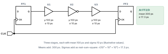
Let us consider the path in Figure 3. Three stages sit between FF1 and FF2. Each stage has a mean of 100 ps and a sigma of 10 ps.
The tool combines the stages with two rules:
- Means add. The mean arrival is 100 + 100 + 100 = 300 ps.
- Sigmas add as root-sum-square (RSS). Square each sigma, add the squares, then take the square root. The path sigma is √(10² + 10² + 10²) = √300 = 17.3 ps.
Now compare two ways to get a 3-sigma arrival, against a required time of 380 ps. Figure 4 draws both.
- A – add n sigma per stage: 130 + 130 + 130 = 390 ps. The slack is 380 − 390 = −10 ps.
- B – statistical: 300 + 3 × 17.3 = 352 ps. The slack is 380 − 352 = +28 ps.
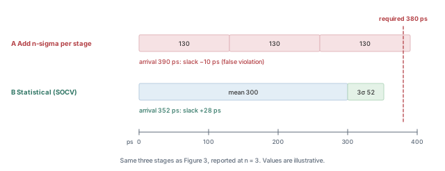
Thus, the statistical answer is less pessimistic, and the gap grows as the path gets deeper. With one stage, both methods agree. With three stages, they differ by 38 ps. With ten stages, as we saw above, they differ by about 205 ps.
1.5 License
SOCV analysis needs the Tempus XL base license. It is not available on Tempus L. If your session runs on Tempus L, plan the license before you plan the analysis, as described in Getting Started with Tempus.
2 Variation data: LVF and .socv files
The tool can only do statistics if the libraries carry sigma values. An ordinary library gives one delay per arc. SOCV needs a second number for each arc – its sigma.
There are two standard sources, plus a bootstrap path for experiments. Figure 5 shows how each one reaches the analysis.
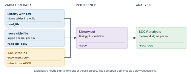
2.1 Liberty Variation Format (LVF)
LVF puts sigma tables directly inside the Liberty .lib file. The library supplier characterizes each cell many times and stores the spread next to the normal delay tables. The main attributes are:
ocv_sigma_cell_riseandocv_sigma_cell_fall– sigma tables for the cell delay, for rising and falling outputs. Rise and fall are separate because the pull-up and pull-down transistors vary differently.sigma_type– which side the table applies to:early,lateorearly_and_late. A library can give one table for both sides, or separate tables when the spread is not symmetric.ocv_derate_distance_group– names a distance-based derate group for the cell.
Because the data lives in the .lib, a plain read_lib loads it. No extra option is needed.
2.2 The .socv side file
A .socv file is a separate text file that holds sigma values next to an ordinary library. Teams use it when the timing library has no LVF, or when the sigma data comes from a different source.
Each entry follows a logical order. It first names the object, then the timing arc, then the conditions, and finally the sigma values. Table 2 lists every attribute.
| Group | Attribute | What it describes |
|---|---|---|
| Object | object_type |
The kind of object the entry applies to |
| Object | object_spec |
Which object, for example a library cell |
| Arc | pin, pin_direction |
The pin of the arc and its direction |
| Arc | related_pin, related_direction |
The related (input or clock) pin and its direction |
| Arc | type |
delay, slew, setup, hold, recovery or removal |
| Conditions | when |
The logic condition of the arc |
| Conditions | related_transition |
The transition on the related pin |
| Conditions | output_loading |
The output load points of the table |
| Conditions | constraint_transition |
The transition axis for timing-check entries |
| Value | sigma |
The sigma values |
| Distance | late_distance, late_distance_derate |
Distance points and derates for the late side |
| Distance | early_distance, early_distance_derate |
Distance points and derates for the early side |
Let us read the table as a story. An entry first picks a cell with object_spec. It then picks the arc from related_pin to pin, and its type, such as delay. Finally, it gives the conditions and the sigma values. The distance attributes then add separate derates that depend on distance, for the late and early sides. Figure 6 draws the same story as five steps.
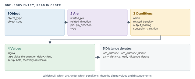
type attribute decides what the sigma varies – a delay, a slew or a timing check.Note that type covers more than delay. Sigma can also apply to slew and to setup, hold, recovery and removal checks. Thus, a full .socv file varies the timing checks too, not only the path delays.
2.3 Loading the data
The load command depends on the data format and on how the session is built. In a single-corner session, read_lib loads both forms:
tempus> read_lib -socv [list libA.socv libB.socv]    ;# .socv side files
tempus> read_lib [list libA-LVF.lib libB-LVF.lib]    ;# Liberty with LVF tables
read_lib -socv– reads.socvside files. The timing libraries themselves are read as usual.read_libwith LVF libraries – reads the timing data and the sigma tables together.
In an MMMC session, the .socv files belong to a library set. Each set then carries its own variation data for its corner:
tempus> create_library_set -name libsetMax \
          -timing [list lib1.lib lib2.lib] \
-socv [list lib1.socv lib2.socv] ;# timing libs plus sigma filesA library set takes -aocv or -socv data, not both. Multi-mode multi-corner setup is covered in Multi-Mode Multi-Corner Analysis.
2.4 Bootstrapping from AOCV tables
Sometimes a team has AOCV tables but no sigma data yet. The tool can infer sigma from the AOCV tables. This is meant for experiments only, and it models delay variation only.
Why would anyone do this? It answers an early planning question: how much slack would SOCV give back? The team can measure that before paying for full sigma characterization.
Both settings must come before any library is read:
tempus> set timing_library_infer_socv_from_aocv true        ;# build sigma from AOCV
tempus> set timing_library_scale_aocv_to_socv_to_n_sigma 3  ;# AOCV value treated as 3 sigma
tempus> read_lib -aocv myDerates.aocv.lib                   ;# or create_library_set -aocv
timing_library_infer_socv_from_aocv true– tells the tool to turn AOCV tables into sigma data as they are read.timing_library_scale_aocv_to_socv_to_n_sigma– says how many sigmas an AOCV derate stands for. With 3, the tool treats each AOCV value as a 3-sigma point.read_lib -aocvorcreate_library_set -aocv– then loads the AOCV tables in the usual way.
If the settings come after the libraries, the libraries are already loaded without sigma. The inference then has nothing to work on. Figure 7 shows the correct order and both limits.
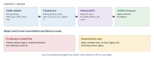
Signing off with AOCV-inferred sigma. It covers delay variation only, so slew and timing-check variation are missing. Use it to estimate the gain from SOCV, then switch to real LVF or .socv data.
.lib or from a .socv side file. AOCV inference is a quick experiment, set before any library is read.3 Enabling and tuning SOCV analysis
3.1 Turning SOCV on
Loading sigma data does not change the analysis by itself. The tool still times with single numbers until SOCV is switched on. One command does that:
tempus> set_analysis_mode -socv true -analysisType onChipVariation -cppr both
;# statistical OCV with CPPR for setup and hold-socv true– use mean and sigma for every arc that has variation data. Arcs without data typically keep a sigma of 0.-analysisType onChipVariation– SOCV builds on on-chip variation analysis. Early and late values are still used for launch and capture, as in Analysis Modes, CPPR and AOCV.-cppr both– remove clock pessimism for both setup and hold. Without it, the shared part of the clock tree gets both an early and a late value, which adds pessimism.
3.2 The statistical min/max mode
When two paths meet at a gate, the tool must pick one arrival to carry forward. For setup it takes the later one, and for hold the earlier one. With single numbers, this is easy: 300 ps is later than 290 ps.
With distributions, "the later one" needs a rule. Let us say path A has mean 300 ps and sigma 5 ps. Path B has mean 290 ps and sigma 20 ps. At 3 sigma, A reaches 315 ps but B reaches 350 ps. Which one is "later" depends on how we look. The global timing_socv_statistical_min_max_mode sets this rule. Figure 8 draws the two arrivals.
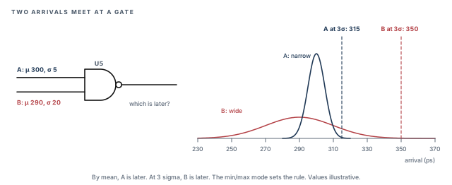
tempus> set timing_socv_statistical_min_max_mode mean_and_three_sigma_bounded
                                       ;# bound the result by mean and 3-sigma values
Two values are in common use, mean_and_three_sigma_bounded and three_sigma_bounded. As the names suggest, the first bounds the result using both the mean and the 3-sigma values. The second bounds it using the 3-sigma values. Many example scripts use three_sigma_bounded. Confirm the default and all allowed values with help in your installation before choosing.
3.3 Choosing n for reports
Reports show each value as mean + n × sigma. The command set_socv_reporting_nsigma_multiplier sets n for a check type, here setup, and can limit it to one view.
tempus> set_socv_reporting_nsigma_multiplier -setup 2.5 -view std_max_setup
;# setup reports at mean + 2.5 sigma-setup 2.5– the n used for setup checks. Other check types typically have their own option; confirm the list withhelp set_socv_reporting_nsigma_multiplier.-view std_max_setup– limits the setting to one analysis view, so each corner can use a different n.
Let us see the effect on the path from Figure 3. At n = 3, the arrival is 300 + 3 × 17.3 = 352 ps. At n = 2.5, it is 300 + 2.5 × 17.3 = 343.3 ps. The slack against 380 ps grows from 28 ps to 36.7 ps. Figure 9 marks both points on the arrival distribution.
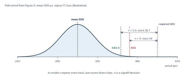
A smaller n reports less pessimistic numbers. However, it also covers fewer chips. Thus, n is a signoff decision, agreed with the foundry and the project team. It is not a knob to turn when a path fails.
3.4 Verbose statistical reports
By default, a report shows the final n-sigma values. To see the mean and sigma behind each value, turn on verbose mode:
tempus> set timing_report_enable_verbose_ssta_mode true ;# add mean and sigma detailTurn on verbose mode while you learn SOCV and while you debug a surprising path. It shows whether a large value comes from the mean or from the sigma. A large mean points to a slow cell or a long wire. A large sigma points to a cell with high variation, typically a weak or low-voltage cell.
set_analysis_mode -socv true, choose the min/max mode, and set the reporting n for setup, per view if needed.4 Reading SOCV reports
4.1 What the numbers mean
Every delay, slew and arrival in an SOCV report is shown as mean + n × sigma. However, the arrival column does not equal the sum of the delay column. This surprises almost everyone the first time.
Let us return to Figure 3 at n = 3. Each stage shows 130 ps. A beginner expects the arrival to reach 390 ps. The tool shows 352 ps instead, because it adds the means and combines the sigmas by RSS. The excerpt below walks through it stage by stage.
# Delay and Arrival columns show mean + 3 sigma
Pin        Delay   Arrival   Arr. mean   Arr. sigma
FF1/Q        -       0.0
U1/Y       130.0   130.0       100         10.0
U2/Y       130.0   242.4       200         14.1
U3/Y       130.0   352.0       300         17.3
Read it row by row:
- After U1, the arrival has mean 100 ps and sigma 10 ps. At 3 sigma, that is 130 ps.
- After U2, the mean is 200 ps. The sigma is √(10² + 10²) = 14.1 ps, so the arrival is 200 + 42.4 = 242.4 ps.
- After U3, the mean is 300 ps. The sigma is 17.3 ps, so the arrival is 300 + 52 = 352 ps.
Figure 10 draws these three rows as bars, next to the simple sums a beginner expects.
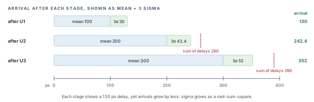
Adding the delay column by hand and reporting a tool bug. In SOCV, arrivals never add exactly. Check the mean and sigma columns instead.
Figure 11 shows the same result as a timing diagram at the capture flop.
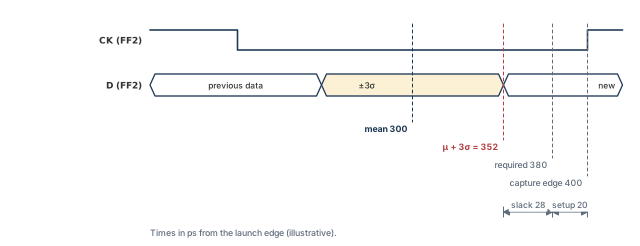
In this illustrative case, the capture edge is at 400 ps and setup needs 20 ps. Thus, the required time is 380 ps. The slack is the gap between the 3-sigma arrival and the required time.
4.2 Report fields
With verbose mode on, these fields can appear in timing reports:
delay_mean,delay_sigma– the mean and sigma of each arc delay.slew_mean,slew_sigma– the mean and sigma of each slew. Slew sigma matters because a varying slew changes the next stage's delay.arrival_mean,arrival_sigma– the mean and sigma of each arrival, after RSS combining.
4.3 Timing properties
Scripts can read the same data as properties. This is useful when you want to sort paths by sigma, or flag cells with high variation. The names follow a pattern:
- Arc properties:
delay_{mean|sigma}_{max|min}_{rise|fall}. For example,delay_sigma_max_riseis the late sigma of a rising arc. - Pin properties:
arrival_*,slack_{mean|sigma}_{max|min}[_{rise|fall}]andslew_*. For example,slack_mean_maxis the mean of the setup slack.
The braces list the choices, and you pick one from each group. The rise/fall part of the slack name is optional, as the brackets show. Thus, slack_sigma_min_fall and slack_sigma_min are both valid names.
5 What carries sigma, and what does not
5.1 The traps
SOCV is only as good as the inputs that carry variation. Several inputs and outputs carry no sigma, or carry only part of it. None of them raises an error. Table 3 lists them.
| Item | What happens in SOCV | What to do |
|---|---|---|
| Values from SDC | Sigma is 0 | Do not expect SDC delays or uncertainty to vary statistically |
set_timing_derate |
Scales both mean and sigma | Use -mean or -sigma to derate only one |
read_sdf |
Annotates the mean only | Do not expect sigma on SDF-annotated arcs |
write_sdf |
Writes mean + n × sigma | Add -no_variation for mean-only delays |
report_delay_calculation |
Shows the mean by default | Remember the value is not the n-sigma delay |
Let us go through them one by one.
- SDC values. An input delay or a clock uncertainty is a fixed number. It has no spread, so its sigma is 0. Any margin you want there must be in the mean value itself.
- Derates. A derate multiplies a delay. By default it multiplies both parts. This is covered below with numbers.
- SDF input. An SDF file holds one delay per arc. Thus,
read_sdfcan only set the mean, and annotated arcs lose their sigma. - SDF output.
write_sdfwrites the n-sigma value, which is pessimistic for simulation. Add-no_variationto write the mean only. - Delay calculation report.
report_delay_calculationshows the mean by default. Its number will not match the n-sigma value inreport_timing.
5.2 The derate trap in numbers
Let us look at the derate trap. Assume a cell with mean 100 ps and sigma 10 ps, and a late derate of 1.05. Figure 12 compares the two outcomes at n = 3.
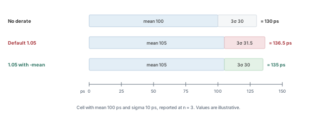
- Default: the mean becomes 105 ps and the sigma becomes 10.5 ps. At 3 sigma, the delay is 105 + 31.5 = 136.5 ps.
- With
-mean: the mean becomes 105 ps and the sigma stays 10 ps. At 3 sigma, the delay is 105 + 30 = 135 ps.
The difference looks small on one cell. On a long path, the extra sigma adds up and can hide real slack. If you only wanted extra margin on the mean, use -mean:
tempus> set_timing_derate -late -cell_delay 1.05 -mean ;# scale the mean, keep sigmaSimilarly, -sigma scales only the sigma. This is useful when the foundry asks for extra variation margin, but not a slower mean.
Writing SDF from an SOCV session for gate-level simulation without thinking. The file holds mean + n × sigma delays. If the simulation needs nominal delays, use write_sdf -no_variation.
5.3 Via variation
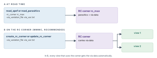
Vias also vary. A via is the small vertical link between two metal layers, and its resistance changes from chip to chip. A via variation file adds that effect to the parasitics. It is given per RC corner:
tempus> read_spef -rc_corner rc_max -via_variation_file via_var.txt top.spef.gz
;# SPEF plus via variation for rc_max-rc_corner rc_max– the RC corner that the parasitics and the via data belong to.-via_variation_file via_var.txt– the file with the via variation values.
The same option exists on read_parasitics. In MMMC sessions, attach the file to the RC corner with create_rc_corner -via_variation_file or update_rc_corner -via_variation_file. It is better to attach it to the corner, because the data then follows the corner into every view that uses it. Figure 13 compares the two ways.
6 Wire variation
6.1 The concept
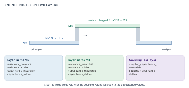
Cells are not the only things that vary. The width and thickness of each metal layer vary from chip to chip. A wider wire has lower resistance (R) and higher capacitance (C). Thus, wire R and C vary too, and each layer varies on its own.
Why on its own? Each metal layer is made in a separate set of process steps. One layer can come out slightly thick on a wafer, while the next comes out slightly thin. Thus, a net that uses two layers sees two separate sources of variation.
Let us consider the net in Figure 14. It starts on M2, climbs to M3 through a via and comes back down. If M3 is slightly thicker on one chip, only the M3 part of the net changes.
6.2 Why it is path-based only
Wire variation applies only in path-based analysis (PBA). It does not apply to graph-based analysis (GBA), exhaustive PBA or infinite PBA.
Here is the short version of the difference. GBA times every pin once, with worst-case slews merged from all paths. PBA then retimes selected paths one at a time, with the real slews of each path. Wire variation is applied during this retiming step. Path-based analysis is covered in detail in Path-Based and Robustness Analysis.
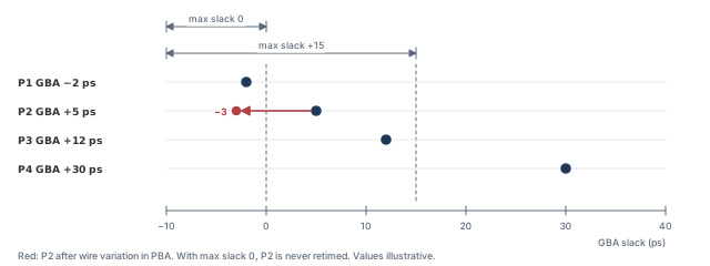
Because only retimed paths see wire variation, the path list matters. Report with a high -nworst and a maximum slack above 0. Otherwise, a path that looks safe in GBA could hide a wire-variation violation. For example, a path with +5 ps of GBA slack is not retimed if the slack limit is 0. Wire variation could have pushed it to −3 ps. Figure 15 shows this case.
6.3 The inputs
Wire variation needs two inputs.
1. An extended SPEF. A normal SPEF lists resistors and capacitors, but not the layer each one is on. The tool needs the layer to apply the right variation. Thus, the parasitics must record the layer of each resistor:
- A
*LAYER_MAPsection maps layer numbers to layer names. - Each resistor carries a
$LAYER=tag that names its layer.
2. A wire variation side file. It lists the variation per layer. Table 4 lists its fields.
| Field | Meaning |
|---|---|
version |
Format version of the file |
layer_name |
The layer the following values apply to |
resistance_meanshift, resistance_stddev |
Shift of the mean and standard deviation of resistance |
capacitance_meanshift, capacitance_stddev |
Shift of the mean and standard deviation of capacitance |
coupling_capacitance_meanshift, coupling_capacitance_stddev |
The same for coupling capacitance |
Each quantity has two numbers, and they do different jobs:
- A mean shift moves the center of the distribution. It says the layer is, on average, a little different from the extracted value.
- A standard deviation sets the spread around that center. It feeds the sigma of the wire delay.
If the coupling values are missing for a layer, the tool uses that layer's capacitance values for coupling as well. Thus, a short side file still works, but coupling then varies with the same values as ground capacitance.
6.4 The flow
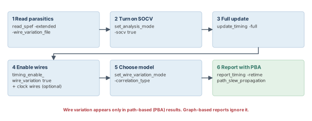
Figure 16 shows the six main steps of a wire variation run. Step 4 also notes the optional clock-wire setting.
tempus> read_spef -extended top.spef.gz -wire_variation_file wireVar.txt
                                                   ;# layer-tagged SPEF plus side file
tempus> set_analysis_mode -socv true               ;# wire variation builds on SOCV
tempus> update_timing -full                        ;# full timing update
tempus> set timing_enable_wire_variation true      ;# turn wire variation on
tempus> set timing_disable_retime_clock_path_slew_propagation false
                                                   ;# let clock wires vary too
tempus> set_wire_variation_mode -correlation_type statistical \
          -rc_correlation_factor -1                ;# statistical model, R-C correlation -1
tempus> report_timing -retime path_slew_propagation ;# path-based report with wire variation
Let us walk through the script, using the step numbers of Figure 16:
read_spef -extended ... -wire_variation_file– reads the layer-tagged parasitics and the per-layer variation in one step.set_analysis_mode -socv true– wire variation produces sigma values, so it needs statistical analysis.update_timing -full– a full update builds the graph-based timing that PBA starts from.timing_enable_wire_variation true– turns wire variation on for retimed paths. The optionaltiming_disable_retime_clock_path_slew_propagation falsebelongs to this step. By default, clock-path wires do not vary in retiming; setting this global tofalseadds variation to clock wires as well.set_wire_variation_mode– chooses the model, explained next.report_timing -retime path_slew_propagation– runs PBA on the reported paths, where wire variation is applied.
6.5 Choosing the model
The command set_wire_variation_mode has two main options.
-rc_correlation_factor– the correlation between the R and C variations. The allowed values are-1and1. Physically, a wider wire lowers R but raises C, so R and C often move in opposite directions. A value of-1typically models that case. Confirm its exact meaning withhelp set_wire_variation_mode.-correlation_type– how the layer variations are combined:statisticalorbinomial.
The two correlation types behave very differently:
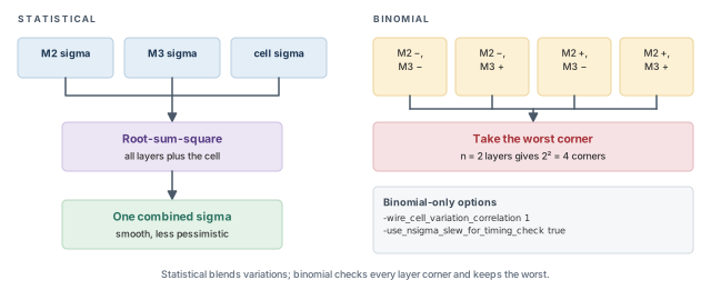
- Statistical – the tool combines the layer variations and the cell sigma by RSS. The result is smooth and less pessimistic.
- Binomial – the tool evaluates the worst of 2ⁿ corners, where each layer is pushed up or down. This is more pessimistic and more like a corner-based check.
Figure 17 compares the two correlation types, and lists the options that apply only to binomial mode.
Let us compare them on a simplified example. A stage has a cell sigma of 12 ps. Its M2 part adds 4 ps of wire sigma, and its M3 part adds 3 ps.
- Statistical: √(12² + 4² + 3²) = √169 = 13 ps.
- Binomial: the worst layer corner pushes both layers the slow way, giving 4 + 3 = 7 ps of wire effect. With the default RSS combination with the cell, √(12² + 7²) = 13.9 ps.
These numbers are illustrative and simplified. They show the trend: binomial is more pessimistic, because the worst corner adds the layers linearly.
Binomial mode has two extra options:
-wire_cell_variation_correlation 1– treat wire and cell variation as fully correlated, so they add linearly. The default is 0, which combines them by RSS. In the example above, a value of 1 would give 12 + 7 = 19 ps.-use_nsigma_slew_for_timing_check true– use the n-sigma slew for timing checks. The default isfalse. This typically adds slew variation to setup and hold checks, which is more pessimistic.
tempus> set_wire_variation_mode -correlation_type binomial \
          -wire_cell_variation_correlation 1 \
-use_nsigma_slew_for_timing_check true ;# worst corner, linear wire+cellStart with the statistical model, because it matches how SOCV treats cells. Use binomial when the signoff rules ask for a corner-style check, and expect smaller slack.
6.6 Reading the results
Wire variation adds its own report fields:
retime_slew_wire_stddev– the wire part of the slew standard deviation.retime_delay_wire_stddev– the wire part of the delay standard deviation.arrival_wire_stddev– the wire part of the arrival standard deviation.
These fields answer one question: how much of the variation comes from metal? Compare arrival_wire_stddev with the total arrival sigma. A large share means the path is sensitive to wires, not cells.
To see the delay calculation details at chosen pins of a retimed path, use report_timing -retime_delaycal_pins with the pin list.
tempus> report_timing -retime path_slew_propagation -retime_delaycal_pins {U2/A U3/A}
;# show retimed delay calculation at two pinsExpecting wire variation in a normal report_timing. Without -retime, the report is graph-based, and wire variation does not apply.
7 Worked example: a statistical signoff run
Let us join the pieces in one session. The assumptions are written as comments at the point of use. After each step, we note what to check before moving on.
The task. A block has one setup view, std_max_setup. The libraries ship with LVF. The foundry asks for setup at 3 sigma, and the project wants per-layer wire variation on the critical paths.
Step 1 – load libraries with variation
# Assuming LVF tables are inside both .lib files
tempus> read_lib [list std_ss-LVF.lib mem_ss-LVF.lib]   ;# LVF is read with the timing data
Because LVF lives inside the .lib, no -socv option is needed. Check the log for library warnings. A library without LVF typically leaves its cells with a sigma of 0, and no error is raised.
Step 2 – load the design and parasitics
tempus> read_verilog top.v                ;# netlist
tempus> set_top_module top                ;# link the design
tempus> read_sdc top.sdc                  ;# constraints (these values carry no sigma)
tempus> read_spef -extended top.spef.gz -wire_variation_file wireVar.txt
                                          ;# layer tags plus per-layer variation
The SPEF must come from an extraction run that writes layer tags. If the extended form is missing, wire variation has no layers to work with.
Step 3 – turn on SOCV and set reporting
tempus> set_analysis_mode -socv true -analysisType onChipVariation -cppr both
                                          ;# statistical OCV with CPPR
tempus> set timing_socv_statistical_min_max_mode mean_and_three_sigma_bounded
                                          ;# rule for statistical max and min
tempus> set_socv_reporting_nsigma_multiplier -setup 3 -view std_max_setup
                                          ;# foundry asks for 3 sigma on setup
tempus> set timing_report_enable_verbose_ssta_mode true   ;# show mean and sigma
Here n is 3 because the foundry asked for it. It is not tuned to make paths pass.
Step 4 – graph-based check first
tempus> update_timing -full               ;# full update with SOCV
tempus> report_timing -nworst 50          ;# GBA view of the worst paths
Assume a path shows a mean arrival of 300 ps and a sigma of 17.3 ps. At n = 3, the arrival is 352 ps. With a required time of 380 ps, the slack is +28 ps.
Before going on, check two things in the verbose fields. First, every cell on the path should have a non-zero sigma. Second, the arrival should match mean + 3 × sigma, not the sum of the delays.
Step 5 – add wire variation on retimed paths
tempus> set timing_enable_wire_variation true                ;# enable wire variation
tempus> set timing_disable_retime_clock_path_slew_propagation false
                                                             ;# vary clock wires too
tempus> set_wire_variation_mode -correlation_type statistical \
          -rc_correlation_factor -1                   ;# statistical model
tempus> report_timing -retime path_slew_propagation -nworst 50
                                                             ;# PBA with wire variation
Now check the arrival_wire_stddev field on the critical path. Assume it is 9 ps, while the total arrival sigma grows to about 19.5 ps (illustrative). Assume also that no layer has a mean shift. Then the slack at 3 sigma drops by about 6.6 ps, from +28 ps to about +21 ps.
If the wire part is a large share of the total sigma, the path is sensitive to metal variation. Thus, a reroute on a different layer may help more than a cell upsize.
In practice, add a maximum slack limit above 0 to the PBA report. This keeps nearly-passing paths in the list, since wire variation can push them negative.
8 Common mistakes and how to catch them
Table 5 gathers the mistakes from this chapter. Each row gives the symptom you would see first.
| Symptom | Likely cause | Fix |
|---|---|---|
| SOCV cannot be enabled | Session runs on Tempus L | Use Tempus XL |
| Sigma is zero on every cell | Libraries have no LVF and no .socv was loaded |
Load LVF libraries or add read_lib -socv |
| AOCV inference has no effect | Settings applied after libraries were read | Set both inference globals before any read_lib |
| Arrival is not the sum of the delays | Expected behavior: means add, sigmas RSS | Read arrival_mean and arrival_sigma |
| Derate changed the sigma too | set_timing_derate scales mean and sigma |
Add -mean or -sigma |
| SDF-annotated arcs show no variation | read_sdf annotates the mean only |
Expect it, or calculate those arcs instead |
| Simulation delays look pessimistic | write_sdf wrote mean + n × sigma |
Use write_sdf -no_variation |
report_delay_calculation disagrees with the report |
It shows the mean by default | Compare with the mean field, not the n-sigma value |
| No wire variation in reports | Graph-based report, or wire variation not enabled | Enable it and report with -retime path_slew_propagation |
| Clock wires never vary | Clock-path slew propagation in retiming is off by default | Set the clock retiming global from Section 6.4 to false |
| Wire variation hits a near-passing path missed by the report | Low -nworst or slack limit at 0 |
Use a high -nworst and a maximum slack above 0 |
9 Interview preparation
The mean is the average delay across chips; sigma measures how widely the delay spreads.
- A 3-sigma delay is mean + 3 × sigma.
- For mean 100 ps and sigma 10 ps, the 3-sigma delay is 130 ps.
- About 99.7% of chips fall within ±3 sigma of the mean.
Because stage variations partly cancel: means add, but sigmas add as root-sum-square.
- A flat derate assumes every stage is slow at once.
- The gap grows with depth. Take 10 stages with sigma 10 ps each, at 3 sigma.
- The flat margin is 300 ps, but the statistical margin is only about 95 ps.
About 352 ps: mean 300 ps plus 3 × 17.3 ps.
- The path sigma is √(3 × 10²) = 17.3 ps.
- Adding 130 ps three times gives 390 ps, which is pessimistic.
- Against a required time of 380 ps, the slack is +28 ps instead of −10 ps.
No. Each value is mean + n × sigma, and sigmas do not add linearly.
- Check
arrival_meanandarrival_sigmawith verbose mode on. - The mean parts of the delays add up exactly; only the sigma parts do not.
From Liberty LVF tables, or from a separate .socv file loaded with read_lib -socv.
- In MMMC,
.socvfiles attach to a library set withcreate_library_set -socv. - AOCV tables can be converted for experiments, covering delay variation only.
The globals were set after the libraries were read; they must come before any library read.
- Inference happens while the AOCV tables are read.
- Once libraries are loaded without sigma, setting the globals later changes nothing.
set_socv_reporting_nsigma_multiplier control?The n used to report values as mean + n × sigma, for a check type such as setup, optionally per view.
- Example:
-setup 2.5 -view std_max_setup. - A lower n gives more slack but covers fewer chips, so n is a signoff decision.
SDC values have sigma 0, read_sdf annotates the mean only, and report_delay_calculation shows the mean by default.
set_timing_deratescales both mean and sigma unless-meanor-sigmais used.write_sdfwrites mean + n × sigma unless-no_variationis used.- None of these raises an error, so they must be known in advance.
report_timing show no wire variation?Wire variation applies only to path-based analysis, not to graph-based results.
- Report with
-retime path_slew_propagation. - It also does not apply to exhaustive or infinite PBA.
- Use a high
-nworstand a slack limit above 0 so near-passing paths are retimed.
An extended SPEF with a *LAYER_MAP and $LAYER= tags, plus per-layer mean shift and standard deviation for R, C and coupling C.
- The layer tags tell the tool which variation applies to each resistor.
- Missing coupling values fall back to the capacitance values.
Statistical combines layer and cell variation by RSS; binomial takes the worst of 2ⁿ layer corners.
- Binomial is more pessimistic, because the worst corner adds layers linearly.
- Binomial can also correlate wire and cell variation fully with
-wire_cell_variation_correlation 1. - Its default of 0 combines wire and cell by RSS.
Chapter recap
Key takeaways
- SOCV stores each delay as a mean and a sigma. Means add, sigmas add as root-sum-square.
- Deep paths gain the most, because flat derates assume every stage is slow at once.
- Sigma comes from LVF or
.socvdata. AOCV inference is for experiments, set before any library read. - Reports show mean + n × sigma, and arrivals are not sums of the delay column.
- SDC values, SDF input and derates need care, because they carry no sigma or affect it in hidden ways.
- Wire variation adds per-layer R and C effects, but only in path-based analysis.
Command recap
| Command or setting | Purpose |
|---|---|
read_lib -socv, create_library_set -socv |
Load .socv sigma data |
timing_library_infer_socv_from_aocv, timing_library_scale_aocv_to_socv_to_n_sigma |
Infer sigma from AOCV tables |
set_analysis_mode -socv true -analysisType onChipVariation -cppr both |
Turn on SOCV |
timing_socv_statistical_min_max_mode |
Rule for statistical max and min |
set_socv_reporting_nsigma_multiplier |
n used in reports, for setup and per view |
timing_report_enable_verbose_ssta_mode |
Show mean and sigma detail |
set_timing_derate -mean, -sigma |
Derate only one part |
write_sdf -no_variation |
Mean-only SDF |
-via_variation_file |
Via variation on SPEF or RC corner |
read_spef -extended -wire_variation_file |
Layer-tagged SPEF plus wire variation data |
timing_enable_wire_variation |
Turn on wire variation |
timing_disable_retime_clock_path_slew_propagation |
Set to false to vary clock wires |
set_wire_variation_mode |
Model, R-C correlation and binomial options |
report_timing -retime path_slew_propagation, -retime_delaycal_pins |
PBA report and delay-calculation detail |
Compact glossary
| Term | Meaning |
|---|---|
| Mean (μ) | The average delay across many chips |
| Sigma (σ) | Standard deviation; how widely the delay spreads |
| n sigma | Mean + n × sigma, the value shown in reports |
| RSS | Root-sum-square: the square root of the sum of squares |
| SOCV | Statistical on-chip variation: timing with mean and sigma |
| LVF | Liberty Variation Format: sigma tables inside a .lib |
| .socv file | A side file holding sigma values for a library |
| Via variation | Chip-to-chip variation of via resistance, given per RC corner |
| Wire variation | Per-layer variation of wire resistance and capacitance |
| Mean shift | A change in the center of a layer's R or C distribution |
| Extended SPEF | SPEF with a layer map and per-resistor layer tags |
| Binomial model | Wire model that keeps the worst of 2ⁿ layer corners |
| GBA | Graph-based analysis: each pin timed once with merged worst slews |
| PBA | Path-based analysis: selected paths retimed with their own slews |
Practical perspective
On advanced nodes, SOCV is often the default signoff method. The usual fight is not about the commands. It is about the inputs. Does every library have LVF? Which n does the foundry require? Do SDF or derates quietly drop sigma?
Thus, check the data first and the margins second. A missing sigma looks like good news in a report, which is exactly why it is dangerous. Wire variation then shows which critical paths depend on metal, which guides reroutes during ECO.
What comes next
So far we have timed one view at a time. Real signoff covers many corners and modes together. In the next chapter, Multi-Mode Multi-Corner Analysis, we build library sets, RC corners, delay corners and views. Then we run them concurrently or distributed.