Chapter overview
A chip must work at every voltage, temperature and process point it will meet in the field. It must also work in every mode – functional, test and low power. Each combination of a corner and a mode is a separate timing problem.
Let us consider a small block with two modes and three corners. That is already six timing runs. Running them one by one wastes hours. It also invites mistakes, because each run is set up by hand and can drift from the others.
Multi-mode multi-corner (MMMC) analysis solves this. You describe each corner and each mode once. The tool then combines them into analysis views and times all of them.
This chapter first builds MMMC inside one session, called concurrent MMMC (CMMMC). It then spreads the same views across several machines, called distributed MMMC (DMMMC). The object model is the same in both. Only the place where the work runs changes.
Learning objectives
- Explain what an analysis view is and why one corner is never enough.
- Build library sets, operating conditions, RC corners and delay corners.
- Bind a different library set and operating condition to a power domain inside a delay corner.
- Create constraint modes and apply typed constraints to several modes at once.
- Predict which SDC commands stay inside one mode and which affect every view.
- Activate setup and hold views, and restrict reports to one view.
- Split a DMMMC run into master, design-load and analysis scripts.
- Save, restore, group and interactively query distributed views.
- Apply the DMMMC rules that prevent socket errors and missing results.
Chapter roadmap
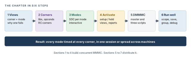
The chapter moves in six steps. Sections 1 to 4 build concurrent MMMC. Sections 5 to 7 distribute it. Figure 1 shows the path. Come back to it whenever you lose your place.
Key commands
Table 1 lists the commands covered in this chapter, grouped by section. Do not try to memorize them now. Each one is explained when it is first needed.
| Section | Command | What it does |
|---|---|---|
| 2 Corners | create_library_set, update_library_set |
Group the libraries used at one corner |
| 2 Corners | create_op_cond, create_opcond, create_timing_condition |
Describe process, voltage and temperature |
| 2 Corners | create_rc_corner |
Describe wire extraction data and scaling |
| 2 Corners | create_delay_corner, update_delay_corner |
Join libraries, conditions and an RC corner |
| 3 Modes | create_constraint_mode, update_constraint_mode |
Attach SDC files to a mode |
| 3 Modes | set_interactive_constraint_modes, get_interactive_constraint_modes, all_constraint_modes |
Apply typed constraints to chosen modes |
| 4 Activate | create_analysis_view, update_analysis_view |
Pair one mode with one delay corner |
| 4 Activate | set_analysis_view, set_default_view, report_analysis_views |
Choose and list the active views |
| 4 Activate | read_mmmc, read_physical, read_netlist, init_design |
Load the views, physical data and netlist |
| 4 Activate | read_spef -rc_corner |
Attach parasitics to one RC corner |
| 4 Activate | report_timing -view, write_sdf -view, save_design |
Report, write and save per view |
| 5 DMMMC | set_distribute_host, set_multi_cpu_usage |
Choose machines and CPUs for clients |
| 5 DMMMC | distribute_read_design, distribute_views |
Load the design and run views on clients |
| 5 DMMMC | merge_timing_reports, exit_servers |
Merge client reports and close clients |
| 6 Run well | distribute_command, get_distribute_variables |
Run a command on clients, read client variables |
| 6 Run well | read_design, read_view_definition, read_power_domain |
Restore one saved view; load views and power intent |
| 6 Run well | set_distribute_mmmc_mode, change_cell |
Query and try changes across views interactively |
1 Why one corner is never enough
1.1 The concept
A corner is one set of physical conditions. It fixes the process point, the supply voltage, the temperature and the wire parasitics. For example, "slow process, 0.9 V, 125 °C, maximum wire capacitance" is one corner.
A mode is one way the chip operates. Functional mode runs the real clocks. Test mode shifts data through scan chains, often with a slower test clock. Each mode is described by its own constraints – its own SDC files.
An analysis view is one corner paired with one mode. It answers one precise question. Does the chip meet timing in this mode, under these conditions? Thus, two modes and two corners give four views.
1.2 Why it matters
Let us consider Figure 2. The same flop-to-flop path is shown at two corners, with a 2.0 ns clock. Assume an ideal clock, so both flops see the edge at the same time.
- At the slow corner, the new data reaches the capture flop at 1.75 ns. Assume a setup time of 0.10 ns. The setup slack is 2.0 − 0.10 − 1.75 = 0.15 ns. A slightly slower corner could make it negative.
- At the fast corner, the new data changes only 0.25 ns after the launch edge. The hold check uses that same edge at the capture flop. Assume a hold time of 0.30 ns. The hold slack is 0.25 − 0.30 = −0.05 ns – a violation.
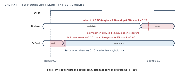
In general, setup is checked at slow corners, where data is latest. Hold is checked at fast corners, where data changes earliest. Every mode adds its own paths and clocks on top. Checking one view would leave the other risks unchecked, and the report would still look clean.
1.3 How the tool organizes views
The design database in Tempus is MMMC-configured by default. Each view is built from a small tree of objects, shown in Figure 3. Let us read it from the top:
- The analysis view points to one constraint mode and one delay corner.
- The constraint mode holds the SDC files.
- The delay corner holds the library data and one RC corner.
- The library data is a timing condition in the common interface, which names one or more library sets. In the legacy interface, the delay corner names the library set and operating condition directly.
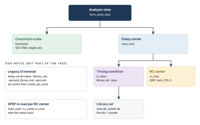
The tree has one big advantage. Each object is defined once and reused. For example, one slow delay corner serves both the functional and the test setup views. If the slow library changes, you edit one library set, and every view that uses it follows.
We will build this tree from the bottom up in the next section.
Multi-corner analysis needs a Tempus XL license. Without it, the tool allows only one setup corner and one hold corner. Getting Started with Tempus lists the license count for each run style, including Tempus L plus ECO for up to eight views.
2 Building the corners
2.1 Library sets
A library set groups the timing libraries used at one corner. A real design rarely has a single library. It may have standard cells, I/O cells and memories, each in its own file. The library set ties them together under one name.
The options are:
-timing– the timing libraries. The first library in the list is the master library. Keep the main standard-cell library first, so the master is the library you expect. Confirm what the master controls withhelp create_library_set.-si– the noise libraries for this corner. Signal integrity analysis reads its cell noise data from them, as Signal Integrity Delay Analysis explains.-aocvor-socv– variation data for that corner. These two are mutually exclusive in one set. A corner uses one variation style, not both.
update_library_set changes an existing set. A common use is to add variation data after the set was first created.
tempus> create_library_set -name slow -timing [list slow.lib pdkIO.lib] ;# master first
tempus> update_library_set -name slow -aocv test.aocv.lib   ;# add AOCV data later
In the legacy flow, the order matters. The libraries are read first. The library sets are then created after the top module is set.
2.2 Operating conditions
An operating condition gives the process, voltage and temperature values for a corner. Libraries are characterized at one condition. An operating condition tells the tool which condition this corner represents.
In the legacy interface, it is created with create_op_cond:
tempus> create_op_cond -name PVT1 -library_file slow.lib -P 1.0 -V 1.2 -T 120 ;# PVT-name– the name other commands use to refer to this condition.-library_file– the library file the condition refers to. Confirm its exact role withhelp create_op_cond.-P,-V,-T– the process factor, the voltage and the temperature. Here the corner is process 1.0, 1.2 V and 120 °C.
In the common interface, the same role is played by create_opcond and create_timing_condition. A timing condition names the library sets used by a corner. Thus, the delay corner refers to a timing condition instead of listing libraries directly. Confirm the options of create_opcond with help create_opcond before using it.
2.3 RC corners
An RC corner describes the wire extraction data for one corner. Wires have resistance (R) and capacitance (C). Both change with temperature and with manufacturing variation, so each corner needs its own wire data.
In the common-interface example later in this chapter, the RC corner takes three inputs:
-cap_table– a capacitance table file.-qrc_tech– the QRC technology file used for extraction.-temperature– the temperature for this RC corner, for example 125 for a hot corner and 0 for a cold one.
The RC corner can also scale the extracted values. Scaling is useful when you want a little extra margin, or when early estimates must be calibrated. The scale options come in groups:
-pre_route_res,-pre_route_cap– scale resistance and capacitance before routing. Before routing, the tool only estimates the wires.-post_route_res,-post_route_cap– scale them after routing, when real wires exist.-post_route_cross_cap– scale coupling capacitance after routing. Coupling capacitance sits between neighbor wires and drives crosstalk.-pre_route_clock_res– scale clock-net resistance before routing.-pre_route_clock_cap,-post_route_clock_cap– scale clock-net capacitance before and after routing.
Figure 4 arranges these options as a grid. Read it by row: each row is one kind of wire value, and each column is one design stage. Two cells are empty, because no option is listed for them.
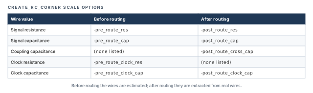
Clock nets have their own factors, so clock wiring can be scaled apart from signal wiring. Confirm the exact value format with help create_rc_corner before using a scale factor.
It is better to leave scale factors at their defaults unless the project has a calibrated reason. A guessed factor hides real problems or creates false ones, and nobody remembers why it was set.
2.4 Delay corners
A delay corner joins the library data and one RC corner. It is the full description of "the conditions" for a view.
Options with -early_ and -late_ prefixes let one corner use different data for early and late paths. Early data is used where the earliest arrival matters, such as hold. Late data is used where the latest arrival matters, such as setup.
update_delay_corner changes a corner later. For example, it can swap the RC corner:
tempus> update_delay_corner -name dc -rc_corner rc ;# dc now uses rc2.5 Power domains inside a delay corner
In a multi-voltage design, one region may run at a different supply. Its cells then need libraries characterized at that voltage. Using the main library for them would give wrong delays.
Figure 5 shows how a delay corner binds a separate library set and operating condition to one power domain. The rest of the design keeps the corner's defaults.
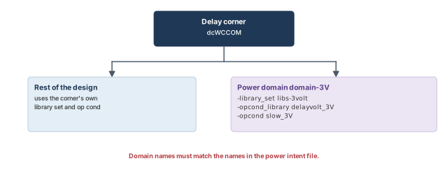
tempus> update_delay_corner -name dcWCCOM -power_domain domain-3V \
-library_set libs-3volt -opcond_library delayvolt_3V -opcond slow_3V ;# 3 V-power_domain– the domain to override. The name must match the name in the power intent.-library_set– the library set for cells in that domain.-opcond_libraryand-opcond– the library that holds the operating condition, and the condition's name.
A designer types domain_3V while the power intent says domain-3V. The binding then does not match the intended domain. Copy domain names from the power intent file instead of retyping them.
2.6 Legacy and common interface
The tool accepts two styles of commands. Older scripts use the legacy interface. Newer scripts use the common interface. Figure 6 compares how each describes the same corner. Each row does the same job, so you can translate a legacy script line by line.
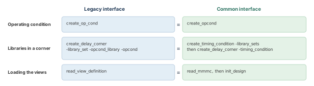
Both styles produce the same object tree. Pick one style per script and stay with it, because mixing them makes scripts hard to read.
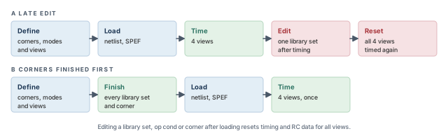
Suppose you edit a library set, an operating condition or a corner after the design is loaded. The tool then resets timing and RC data for all views, which means a long full re-time. Figure 7 shows this in run A. Run B finishes the corners before loading, so the four views are timed once.
3 Constraint modes
3.1 Creating modes
A constraint mode attaches SDC files to one operating mode. For example, a functional mode reads the functional SDC, and a test mode reads the test SDC. The two can define different clocks, different input delays and different exceptions.
tempus> create_constraint_mode -name functional -sdc_files [list eagle.sdc] ;# mode-name– the mode name used by analysis views.-sdc_files– the list of SDC files for this mode.
update_constraint_mode changes the files of an existing mode, for example after the SDC team delivers a new version.
3.2 Typing constraints into several modes
Sometimes you type a constraint at the prompt instead of putting it in a file. For example, you might try a false path while debugging. With several modes, the tool must know which modes the typed constraint belongs to.
Interactive constraint modes set this target, as Figure 8 shows. While a target list is set, every typed constraint goes to each mode in the list.
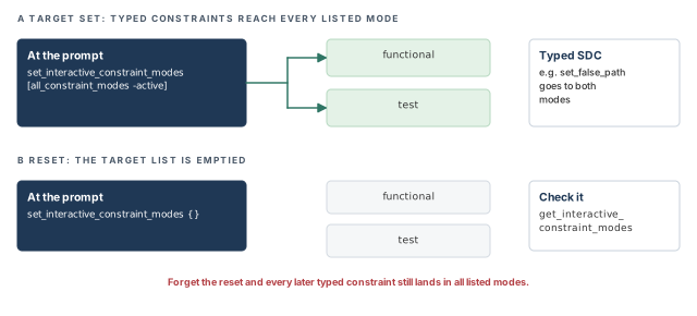
tempus> set_interactive_constraint_modes [all_constraint_modes -active]   ;# target
tempus> set_false_path -from [get_ports scan_en]   ;# illustrative
tempus> set_interactive_constraint_modes {}        ;# stop targeting
tempus> get_interactive_constraint_modes           ;# confirm the target is empty
[all_constraint_modes -active]– returns the modes used by the active views.{}– an empty list ends the targeting.get_interactive_constraint_modes– shows the current target, so you can confirm it.
Always reset the target with an empty list. Otherwise, later typed constraints still go to every listed mode. Interactive constraint modes are not available in DMMMC. There, constraints belong in the SDC files that each client reads.
A typed constraint is easy to forget. When a fix works, move it into the right SDC file. Then the next run gets it too, and the reason stays recorded.
3.3 Isolated SDC and the group_path exception
The SDC of each mode is isolated. A clock created in the test SDC does not exist in the functional views. An input delay in the functional SDC does not touch the test views. This is exactly what we want, because the modes describe different situations.
However, there is one important exception, shown in Figure 9. A path group collects paths so that reports and optimization treat them together. The command group_path is global across views.
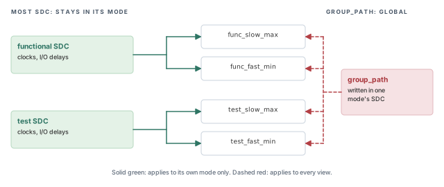
group_path reaches every view.What to notice: A path group written in one mode silently regroups paths in all modes.A designer adds group_path to the test SDC to study scan paths. The functional reports now group paths differently too. It is better to keep path groups in one shared place, because they act across views anyway.
group_path, which is global across views.4 Activating views and reporting
4.1 Creating views
An analysis view pairs a constraint mode with a delay corner. It is the unit that the tool times and reports.
tempus> create_analysis_view -name func_slow_max -constraint_mode functional \
-delay_corner slow_max ;# one mode + one corner-name– the view name. A name that encodes mode and corner, such asfunc_slow_max, makes reports easy to read.-constraint_modeand-delay_corner– the two halves of the view.
update_analysis_view changes the pairing of an existing view later.
4.2 Choosing the active views
Creating a view does not make the tool time it. set_analysis_view chooses the active views. It takes two lists:
-setup– the views checked for setup.-hold– the views checked for hold.
Each list needs at least one view. The first view in each list becomes the default view for that check. Figure 10 shows a common arrangement for two modes and two corners.
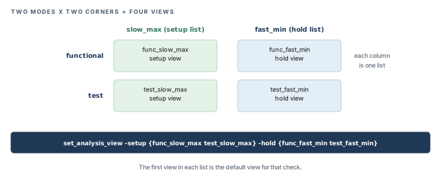
tempus> set_analysis_view -setup {func_slow_max test_slow_max} \
            -hold {func_fast_min test_fast_min}   ;# first in each list is default
tempus> set_default_view func_slow_max             ;# change the default view
tempus> report_analysis_views                      ;# list views and their roles
report_analysis_views is your first check after activation. It lists the views and their roles. If a view you expected is missing, the reports will never show its paths.
4.3 A complete view definition
Let us put the pieces together in the common interface. Read the file below from top to bottom. It builds the object tree of Figure 3 from the leaves up.
- Two library sets: slow and fast.
- Two timing conditions, one per library set.
- Two RC corners: hot at 125 °C and cold at 0 °C.
- Two delay corners, each joining a timing condition and an RC corner.
- One constraint mode.
- Two views and their activation.
Figure 11 shows the same order as a flow, with the loading commands at the end. Each step uses names created by the steps before it, so the order in the file matters.
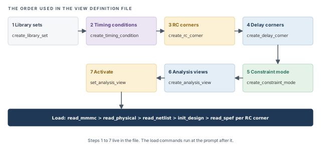
create_library_set -name slow -timing [list slow.lib pdkIO.lib]   ;# slow libraries
create_library_set -name fast -timing [list fast.lib pdkIO.lib]   ;# fast libraries
create_timing_condition -name tc_slow -library_sets [list slow]  ;# slow condition
create_timing_condition -name tc_fast -library_sets [list fast]  ;# fast condition
create_rc_corner -name rc_max -cap_table capTable -qrc_tech qrcTechFile \
    -temperature 125                                              ;# hot wires
create_rc_corner -name rc_min -cap_table capTable -qrc_tech qrcTechFile \
    -temperature 0                                                ;# cold wires
create_delay_corner -name slow_max -timing_condition {tc_slow} \
    -rc_corner rc_max                                             ;# setup corner
create_delay_corner -name fast_min -timing_condition {tc_fast} \
    -rc_corner rc_min                                             ;# hold corner
create_constraint_mode -name functional -sdc_files [list eagle.sdc]   ;# one mode
create_analysis_view -name func_slow_max -constraint_mode functional \
    -delay_corner slow_max                                        ;# setup view
create_analysis_view -name func_fast_min -constraint_mode functional \
    -delay_corner fast_min                                        ;# hold view
set_analysis_view -setup [list func_slow_max] -hold [list func_fast_min]   ;# on
The file is loaded with read_mmmc. The physical data and the netlist follow, and init_design links everything:
tempus> read_mmmc viewDefinition.tcl                ;# corners, modes, views
tempus> read_physical -lef {tech.lef cells.lef}     ;# physical data
tempus> read_netlist top.v.gz                       ;# the netlist
tempus> init_design                                 ;# link everything
4.4 Parasitics, reports and saved sessions
Once the views exist, a few rules decide how data comes in and how results go out:
- SPEF after the views. Read the SPEF only after the views exist. Each file attaches to one RC corner with
-rc_corner. If the RC corner does not exist yet, the file has nowhere to go. - Reports.
report_timingcovers all active views by default. Use-viewto restrict a report to one view, for example while debugging one mode. - SDF.
write_sdf -view <view>writes the delays of one view. A simulation team usually wants one SDF per corner. - Command record. The MMMC configuration is captured in
tempus.cmd. Check this file when you need to trace how a run was set up. - Saved sessions.
save_designkeeps the interactive constraints you typed, together with the session.
tempus> read_spef -rc_corner rc_max slow.spef.gz         ;# after the views exist
tempus> read_spef -rc_corner rc_min fast.spef.gz         ;# one file per RC corner
tempus> report_timing -view func_slow_max                 ;# one view only
tempus> write_sdf -view func_slow_max func_slow_max.sdf ;# SDF for one viewWhen a path fails in one view, report it with -view for that view alone. The output is shorter, and you are not misled by numbers from other corners.
set_analysis_view, read SPEF afterwards, and use -view when you need one view.5 Distributed MMMC
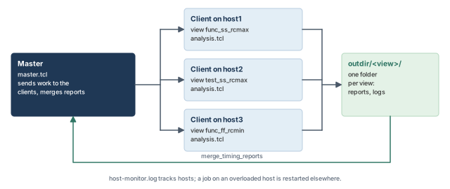
So far, every view ran inside one session. This section moves the same views onto several machines. Figure 12 shows where we are heading: one master and several clients.
5.1 The concept
Concurrent MMMC keeps every view in one process. That works well for a handful of views. With many views on a large design, one machine runs out of memory or the run takes too long.
Distributed MMMC sends each view to its own client process, often on another machine. A master process controls the clients. It hands out the work, waits for results and merges the reports.
The license count follows the views. DMMMC needs one L or XL license for the master and one per view. An XL process gets 16 CPUs, and an L process gets 8. For example, four views need five base licenses in total.
5.2 Three scripts, three jobs
A DMMMC run is split into three scripts. Each has one job. Figure 13 shows how they connect.
- master.tcl – runs on the master. It chooses hosts and CPUs, loads the design on the clients, runs the views, merges reports and exits.
- design_load.tcl – runs on each client first. It reads the design and creates the MMMC objects. It must not contain
read_speforset_analysis_view. - analysis.tcl – runs once per view. It reads the SPEF of every RC corner, sets analysis options and writes reports. Redirected reports land in
<outdir>/<view>/.
Why the strict split? The master decides which view each client runs. Thus, view activation inside a client script would conflict with the master. The SPEF belongs to the analysis step, so each client attaches parasitics to its own corners.
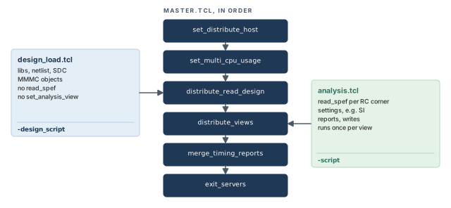
-design_script, and the analysis script with -script.What to notice: SPEF reading and view activation are absent from the design-load script.5.3 Command breakdown: master.tcl
set_distribute_host chooses where clients run. It has three forms:
-rsh -add {host1 host2}– log in to the named machines with rsh. The hosts need passwordless login.-lsf– submit clients to an LSF batch queue.-queuenames the queue,-argspasses submit options such as{-x -W 30}, and-resourcegives the resource request. Confirm the formats withhelp set_distribute_host.-local– run the clients on the local machine. This is handy for small tests.
set_multi_cpu_usage -remoteHost 3 -cpuPerRemoteHost 8 asks for three client hosts with eight CPUs each. With rsh, -remoteHost must not exceed the number of hosts added. This setting also decides how many licenses are requested.
distribute_read_design loads the design on the clients. -design_script names the design-load script, and -outdir names the folder for results.
distribute_views runs the views. -views lists them, and -script names the analysis script.
merge_timing_reports combines one report from each view folder into one report. -view_dirs lists the view folders, and -base_report names the report file to merge from each one. -base_dir is the folder that holds the view folders – typically the -outdir of the run. The merged result is redirected to a file.
exit_servers closes the clients and releases their licenses.
set outDir ./out                                       ;# result folder
set_distribute_host -rsh -add {host1 host2 host3}      ;# client machines
set_multi_cpu_usage -remoteHost 3 -cpuPerRemoteHost 8  ;# 3 clients, 8 CPUs each
distribute_read_design -design_script design_load.tcl -outdir $outDir   ;# load
distribute_views -views {func_ss_rcmax test_ss_rcmax} -script analysis.tcl   ;# run
merge_timing_reports -view_dirs {func_ss_rcmax test_ss_rcmax} \
    -base_report hold_worst.rpt -base_dir $outDir > merged.rpt   ;# one merged report
exit_servers                                                  ;# close the clients
5.4 Command breakdown: analysis.tcl
The analysis script runs inside each client, once per view. It is a normal timing script, with one rule: read the SPEF of every RC corner.
read_spef -rc_corner rcMax slow.spef.gz      ;# every RC corner is read
read_spef -rc_corner rcMin fast.spef.gz      ;# including the other corner
set_delay_cal_mode -SIAware true             ;# analysis setting: SI on
report_timing -machine_readable -max_path 10 -check_type setup > setup.rpt  ;# report
write_sdf x.sdf ; write_sdc c.sdc ; write_eco_opt_db ;# per-view outputs-machine_readablewrites the report in a machine-readable format, which scripts can parse easily.-max_path 10limits the report to ten paths.-check_type setupreports setup checks.- The
write_commands produce one SDF, one SDC and one ECO database per view. - The RC corner names (
rcMax,rcMin) must match the names in the view definition. A name that matches no RC corner leaves that SPEF unattached.
5.5 Watching the clients
The master writes host-monitor.log, which tracks the client hosts. If a host is overloaded, the job is restarted on another host. Thus, when a run takes longer than expected, this log is the first place to look.
6 Running DMMMC well
6.1 Where variables live
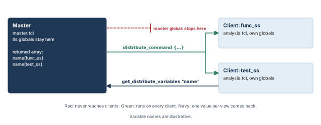
The master and the clients are separate processes. Thus, a variable set in master.tcl exists only in the master. A global setting affects the analysis only if it is set inside a client script.
Let us consider an example. You set an SI global in master.tcl and expect every view to use it. The clients never see it, so the reports come out with the old setting. Nothing warns you.
Two commands bridge this gap:
distribute_command {...}– runs the commands in braces on the clients.get_distribute_variables "name"– reads a client variable back. Give the name without$. The result is an array indexed by view, so each view's value is kept separately.
Figure 14 shows the three paths a setting can take. A global typed in master.tcl stops at the master. distribute_command carries commands to every client, and get_distribute_variables brings values back.
6.2 Saving and restoring
Loading a large design takes time. A distributed run can save each view's session and restore it later, without loading from scratch. Figure 15 shows the two runs.
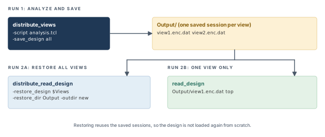
read_design, without any clients.tempus> distribute_views -views $Views -script analysis.tcl -save_design all ;# save
tempus> distribute_read_design -restore_design $Views -restore_dir Output \
-outdir new ;# restore all views
tempus> read_design Output/view1.enc.dat top ;# one view alone-save_design all– saves the session of every view after analysis.-restore_designand-restore_dir– the views to restore and the folder that holds them.-outdir new– a fresh output folder, so the new results do not mix with the old ones.
6.3 Power intent in DMMMC
For a multi-voltage design, the design-load script reads the power intent. Each delay corner then binds its domains, exactly as in Section 2.5. The load order follows Design Import: views, netlist, then the top module.
read_view_definition viewDef.tcl          ;# corners, modes, views
read_verilog top.v                        ;# the netlist
set_top_module top                        ;# link the design
read_power_domain -cpf power.cpf          ;# power intent
update_delay_corner -name dcWCCOM -power_domain domain-3V \
    -library_set libs-3volt -opcond_library delayvolt_3V -opcond slow_3V   ;# 3 V
6.4 Grouping views
Each client can run several views instead of one. Views that share a delay corner group well, because they share the same libraries and parasitics. Figure 16 shows eight views grouped by delay corner.
tempus> distribute_views -combine_num_views 4 -views {v1 v2 v3 v4 v5 v6 v7 v8} \
            -script analysis.tcl                     ;# groups by delay corner
tempus> distribute_views -views {{v1 v2} {v3 v4}} -script analysis.tcl ;# by hand-combine_num_views 4– lets the tool group up to four views per client, by delay corner. This is the recommended form.- Nested lists – you decide the groups yourself. Use this only when you know a better grouping.
Grouped runs write to folders named cmmmc_N. The file views_dir_map.rpt maps each view to its folder, so you can find any view's reports.

6.5 Interactive DMMMC
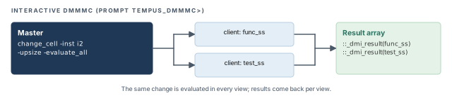
After distribute_views or a restore, you can query all views from one prompt. This is useful to test a fix in every view before committing to it. For example, an upsize can fix setup in a slow view and break hold in a fast view.
tempus> set_distribute_mmmc_mode -views all -interactive true    ;# enter
tempus_dmmmc> change_cell -inst i2 -upsize -evaluate_all        ;# try upsize
tempus_dmmmc> set_distribute_mmmc_mode -views all -interactive false ;# leave- The prompt changes to
tempus_dmmmc>while the mode is on. change_celltakes one of two evaluation switches,-evaluate_allor-evaluate_only. Checkhelp change_cellfor how each behaves.- The result for each view is stored in
::_dmi_result(<view>).
Figure 17 shows one trial change sent to two views.
7 DMMMC rules and troubleshooting
Most DMMMC failures come from a short list of rules. It is better to check them before the run, because a broken distributed run wastes many licenses and hosts at once.
- Read every RC corner in analysis.tcl with
read_spef. A missing corner leaves the views that use it without parasitics. - Never use
set_analysis_viewin DMMMC scripts. The master decides which views run. - Merging happens only on the master, and only into the file you name. Clients never write merged reports.
- Single-machine MMMC and DMMMC cannot coexist in one session. Choose one style per run.
- Merged noise reports lack view names. Keep the per-view noise reports as well, or you cannot trace a noise failure to its view.
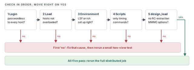
The error "Unable to open socket, connection refused" has five usual causes. Check each one in order:
- Passwordless login to every client host works.
- The client hosts are not overloaded.
- The LSF or rsh environment is set up correctly.
- The scripts contain no non-timing commands.
- design_load.tcl contains no RC-extraction options on MMMC objects.
Figure 18 turns this list into a checklist. Work from left to right, and stop at the first check that fails.
Before a large run, test the setup with two views and -local. A two-view test fails in minutes instead of after a full queue wait.
8 Worked example: four views, two ways
The task. A block has a functional mode and a test mode. It must be checked at a slow corner for setup and at a fast corner for hold. We first run the four views concurrently. Then we run the same views distributed, as we would near tapeout.
Step 1 – describe corners and modes once
The view definition is written once and used by both runs. Notice that there are two modes but only two delay corners. Each corner serves two views. The file has no set_analysis_view, so the same file can also serve the DMMMC design-load script.
# Assuming slow/fast libraries, one cap table and one QRC tech file
create_library_set -name slow -timing [list slow.lib pdkIO.lib]   ;# slow libraries
create_library_set -name fast -timing [list fast.lib pdkIO.lib]   ;# fast libraries
create_timing_condition -name tc_slow -library_sets [list slow]  ;# slow condition
create_timing_condition -name tc_fast -library_sets [list fast]  ;# fast condition
create_rc_corner -name rc_max -cap_table capTable -qrc_tech qrcTechFile \
    -temperature 125                                              ;# hot wires
create_rc_corner -name rc_min -cap_table capTable -qrc_tech qrcTechFile \
    -temperature 0                                                ;# cold wires
create_delay_corner -name slow_max -timing_condition {tc_slow} \
    -rc_corner rc_max                                             ;# setup corner
create_delay_corner -name fast_min -timing_condition {tc_fast} \
    -rc_corner rc_min                                             ;# hold corner
create_constraint_mode -name functional -sdc_files [list func.sdc]   ;# mode 1
create_constraint_mode -name test -sdc_files [list test.sdc]         ;# mode 2
create_analysis_view -name func_slow_max -constraint_mode functional \
    -delay_corner slow_max                                        ;# view 1
create_analysis_view -name func_fast_min -constraint_mode functional \
    -delay_corner fast_min                                        ;# view 2
create_analysis_view -name test_slow_max -constraint_mode test \
    -delay_corner slow_max                                        ;# view 3
create_analysis_view -name test_fast_min -constraint_mode test \
    -delay_corner fast_min                                        ;# view 4
Step 2 – concurrent run
Four views need multi-corner analysis, so we use a Tempus XL license. One XL covers up to eight views; Tempus L plus ECO would also cover them.
tempus> read_mmmc viewDef.tcl                      ;# 4 views described
tempus> read_physical -lef {tech.lef cells.lef}    ;# physical data
tempus> read_netlist top.v.gz                      ;# netlist
tempus> init_design                                ;# link
tempus> set_analysis_view -setup {func_slow_max test_slow_max} \
            -hold {func_fast_min test_fast_min}    ;# activate all four
tempus> read_spef -rc_corner rc_max top_max.spef.gz   ;# after views exist
tempus> read_spef -rc_corner rc_min top_min.spef.gz   ;# second RC corner
tempus> report_analysis_views                      ;# confirm 4 active views
tempus> report_timing -view test_fast_min          ;# look at test hold alone
What to look for:
report_analysis_viewsmust list four active views, two for setup and two for hold.- The test hold report shows only test-mode paths at the fast corner. Scan shift paths often appear here first, because they are short.
Step 3 – the same views, distributed
The design-load script holds Step 1 plus the netlist, but no SPEF and no view activation. The analysis script reads both SPEF files and writes reports. The master ties them together.
# Assuming four rsh hosts with passwordless login
set outDir ./out                                        ;# result folder
set Views {func_slow_max func_fast_min test_slow_max test_fast_min}   ;# all four
set_distribute_host -rsh -add {hostA hostB hostC hostD} ;# client machines
set_multi_cpu_usage -remoteHost 4 -cpuPerRemoteHost 8   ;# 4 <= hosts added
distribute_read_design -design_script design_load.tcl -outdir $outDir   ;# load
distribute_views -views $Views -script analysis.tcl     ;# one client per view
merge_timing_reports -view_dirs $Views -base_report setup.rpt \
    -base_dir $outDir > merged_setup.rpt                 ;# one view of all results
exit_servers                                            ;# release licenses
This run needs five base licenses: one for the master and one per view.
Step 4 – verify
- Confirm that
./outholds a folder for each of the four views. - Check
host-monitor.logfor restarted jobs. A restart is not an error, but it explains a slow run. - Compare
merged_setup.rptwith the concurrent run of Step 2. The worst paths should match, provided both runs use the same analysis settings. The analysis script turns SI on, so turn it on in Step 2 as well before comparing. - Keep each view's noise reports, since a merged noise report has no view names.
9 Common mistakes and how to catch them
Table 2 gathers the mistakes from this chapter. Each row gives the symptom you would see first.
| Symptom | Likely cause | Fix |
|---|---|---|
| Only one setup and one hold corner allowed | No license that enables multi-corner analysis | Use XL, or L plus ECO for up to 8 views |
| All views re-timed after a small edit | Library set, op cond or corner edited after load | Finish corner definitions before loading |
| Power-domain cells use the wrong library | Domain name does not match the power intent | Copy the name from the power intent |
| Path groups change in every mode | group_path placed in one mode's SDC |
Keep path groups in a shared, deliberate place |
| Typed constraint lands in every mode | Interactive modes never reset | Run set_interactive_constraint_modes {} |
| SPEF not attached to a corner | SPEF read before the views existed | Read SPEF after the views, per RC corner |
| A distributed view has no parasitics | One RC corner missing in analysis.tcl | Read every RC corner in analysis.tcl |
| Client ignores a global you set | Global set in master.tcl | Set it in the client script or use distribute_command |
| "Unable to open socket, connection refused" | Login, load, LSF/rsh, non-timing commands or RC options | Check the five causes in Section 7 |
| Merged noise report cannot be traced to a view | Merged noise reports drop view names | Keep the per-view noise reports |
set_analysis_view found in a client script |
Activation copied from a concurrent script | Remove it; the master chooses views |
10 Interview preparation
One constraint mode paired with one delay corner.
- The delay corner holds libraries, conditions and an RC corner.
- The mode holds the SDC files.
- Two modes at two corners therefore give four views.
Slow corners give the latest arrivals, which stress setup; fast corners give the earliest changes, which stress hold.
- Setup compares the latest data with the next capture edge.
- Hold compares the earliest data with the same edge.
- No single corner exposes both risks.
set_analysis_view list mean?It becomes the default view for that check.
- Each list needs at least one view.
set_default_viewchanges the default later.report_analysis_viewsconfirms the result.
group_path to the test-mode SDC. What happens to functional reports?They change too, because group_path is global across views.
- Other SDC commands stay isolated in their mode.
- Path groups belong in one shared, deliberate place.
After the views exist, with one file per RC corner.
- Each file attaches to its RC corner with
-rc_corner. - In DMMMC, every RC corner is read inside analysis.tcl.
Use update_delay_corner -power_domain with -library_set, -opcond_library and -opcond.
- The domain name must match the power intent.
- The rest of the design keeps the corner's defaults.
Timing and RC data are reset for all views.
- The whole design must be re-timed, which is slow on large designs.
- Finish corner definitions before loading.
master.tcl, design_load.tcl and analysis.tcl; design_load.tcl must not contain read_spef or set_analysis_view.
- analysis.tcl runs once per view and reads every RC corner.
- The master only coordinates and merges.
Master variables exist only in the master; globals affect analysis only when set in client scripts.
- Use
distribute_commandto run commands on clients. - Use
get_distribute_variablesto read client values back, as an array by view.
Passwordless login, host load, the LSF or rsh setup, non-timing commands and RC-extraction options in design_load.tcl.
- These five causes cover most cases.
- A small two-view test catches them early.
With -combine_num_views or nested view lists; grouping by delay corner with -combine_num_views is recommended.
- Views on one delay corner share libraries and parasitics.
- Grouped results go to
cmmmc_Nfolders, mapped inviews_dir_map.rpt.
Chapter recap
Key takeaways
- A view is one delay corner plus one constraint mode. Multi-corner analysis needs Tempus XL, or L plus ECO for up to eight views.
- Build library sets, conditions and RC corners, then join them in delay corners. Power domains can override them.
- SDC is isolated per mode, but
group_pathis global. - Finish corner definitions before loading. Later edits reset timing for all views.
- Activate views with
set_analysis_view, read SPEF afterwards, and use-viewfor one view. - DMMMC splits work into master, design-load and analysis scripts, with strict rules for each.
Command recap
| Command | Purpose |
|---|---|
create_library_set, update_library_set |
Libraries for a corner |
create_op_cond, create_opcond, create_timing_condition |
Process, voltage, temperature |
create_rc_corner, create_delay_corner, update_delay_corner |
Wire data and full corners |
create_constraint_mode, update_constraint_mode, set_interactive_constraint_modes |
Modes and typed constraints |
read_mmmc, init_design, read_spef -rc_corner |
Load views and attach parasitics |
report_timing -view, write_sdf -view |
Report or write one view |
create_analysis_view, set_analysis_view, report_analysis_views |
Views and activation |
set_distribute_host, set_multi_cpu_usage |
Client hosts and CPUs |
distribute_read_design, distribute_views, merge_timing_reports, exit_servers |
The DMMMC run |
distribute_command, get_distribute_variables |
Talk to clients |
set_distribute_mmmc_mode, change_cell |
Interactive DMMMC |
Compact glossary
| Term | Meaning |
|---|---|
| Corner | One set of process, voltage, temperature and parasitic conditions |
| Constraint mode | One operating mode, described by its SDC files |
| Analysis view | One constraint mode plus one delay corner |
| Library set | The libraries used at one corner; the first is the master |
| Timing condition | Common-interface object naming the library sets of a corner |
| RC corner | Wire extraction data and scale factors for one corner |
| Delay corner | Library data plus one RC corner |
| Default view | The first view in a setup or hold list |
| CMMMC | Concurrent MMMC: all views in one session |
| DMMMC | Distributed MMMC: views run by clients, controlled by a master |
| Master | The process that runs master.tcl and merges results |
| Client | A process that runs one view or one group of views |
Practical perspective
On a real project, the view definition file is one of the most reused files in the flow. Placement, routing and signoff all read it. Thus, a clean set of corners and modes pays off many times. Distribution becomes important near tapeout, when tens of views must be checked every night.
What comes next
So far, every view has been timed on the full flat design. Large chips are built from blocks, and each block team needs the top-level timing around it. In the next chapter, Hierarchical Timing Context, we pass that top-level context down to a block.